Vector Databases Explained: How Embeddings, Similarity Search, and AI Retrieval Really Work
Imagine asking ChatGPT about a research paper published yesterday.
Not last year.
Not six months ago.
Yesterday.
:: Table of Contents
It reads your question, searches through hundreds of pages of documents, finds the relevant information in seconds, and responds as if it had always known the answer.
But there's a problem.
Large language models don't continuously learn from the internet. Their knowledge is limited by the data they were trained on. Once training finishes, the model's parameters remain fixed until it's retrained or updated.
So where did the answer come from?
It wasn't hidden somewhere inside the billions of parameters of the model.
It wasn't downloaded from Google during your conversation.
And it certainly wasn't memorized during training.
Yet the model still retrieved information it had never seen before.
Modern AI systems solve this puzzle every single day. Customer support assistants answer questions about newly uploaded company manuals. Coding assistants understand repositories created this morning. Legal copilots search contracts written hours ago. Medical assistants retrieve the latest clinical guidelines without retraining the underlying model.
The language model is only one piece of the system.
Behind the scenes, another component is quietly doing most of the work. It stores millions—even billions—of pieces of information, not as paragraphs or rows in a table, but as mathematical representations that can be searched by meaning rather than by exact words.
Ask about "electric vehicles," and it can still find documents that only mention "battery-powered cars."
Search for "heart attack," and it understands that "myocardial infarction" may describe the same concept.
Traditional databases were never designed to solve problems like these.
To understand how modern AI retrieves knowledge, recommends similar content, powers semantic search, and enables Retrieval-Augmented Generation (RAG), we first need to understand the technology that makes it all possible.
The answer isn't a larger language model.
It's an entirely different kind of database.
And once you understand how it works, you'll start seeing it behind almost every modern AI application you use today.
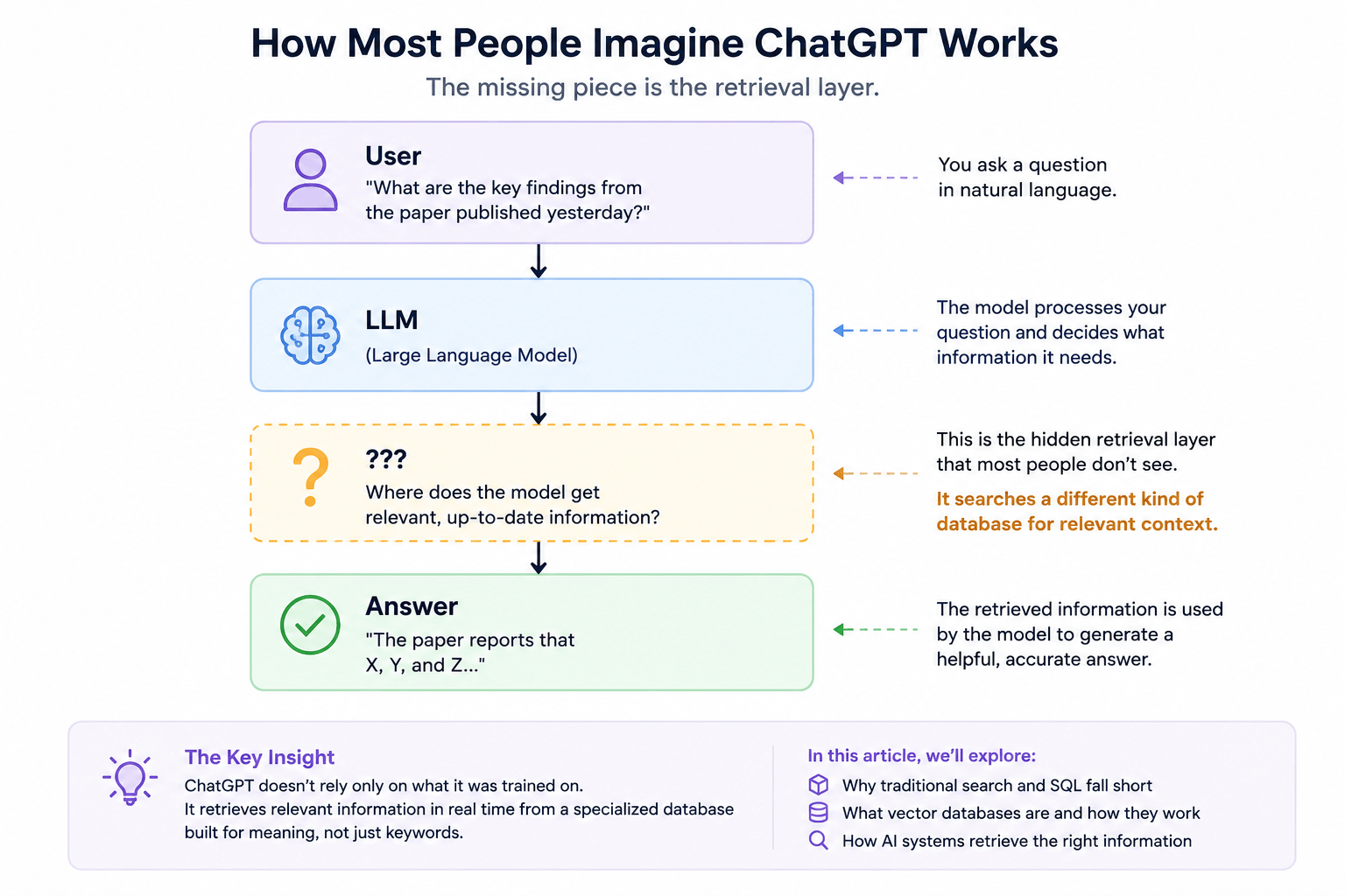
Modern AI systems contain an entire retrieval layer that most users never see. We'll uncover what the "???" represents throughout this article.
1. The Search Problem Nobody Talks About5 min read
Imagine opening Google and searching for:
best car for long road trips
Within milliseconds, Google understands what you're asking. It doesn't simply look for web pages containing the exact words best, car, long, road, and trips. It considers synonyms, context, spelling mistakes, related concepts, and hundreds of other signals before deciding which pages are most relevant.
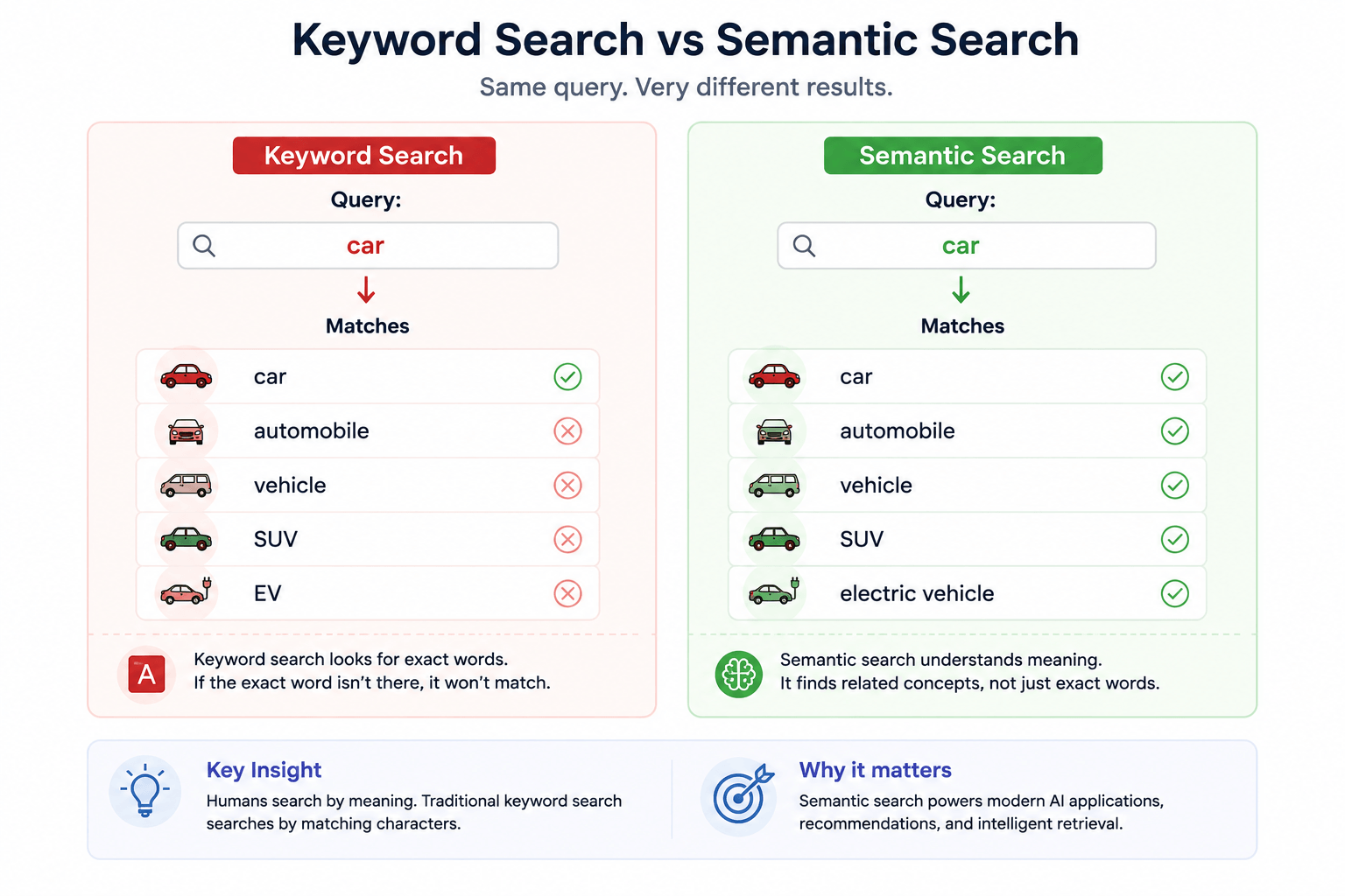
Now imagine performing the same search in a traditional database.
Suppose you have a table containing thousands of automobile articles.
SELECT *
FROM articles
WHERE title LIKE '%car%';1 rows returnedThen
LIKE '%automobile%'0 row returnedNeither article contains the exact phrase "best car for long road trips."
A traditional database doesn't understand that:
- car and automobile often describe the same thing.
- road trip and long-distance travel are closely related.
- SUV is a type of car.
- electric vehicle is another category of automobile.
To the database, these are simply different strings of text.
It has no concept of meaning.
That's because relational databases were never designed to understand language. Their job is to store structured information efficiently and retrieve records that match explicit conditions. If you ask for rows where the title contains the word car, the database will faithfully return rows containing car—and ignore everything else.
Mental Model
SQL doesn't understand ideas.
It understands characters.
For decades, this approach worked perfectly.
Banking systems, inventory management, payroll software, airline reservations, and countless other applications rely on relational databases because structured data has well-defined relationships. Customer IDs match customer records. Product IDs match inventory. Order numbers reference invoices.
Natural language is completely different.
Humans rarely use the exact same words to express the same idea.
Consider these three queries:
- best car for families
- best automobile for families
- best family vehicle
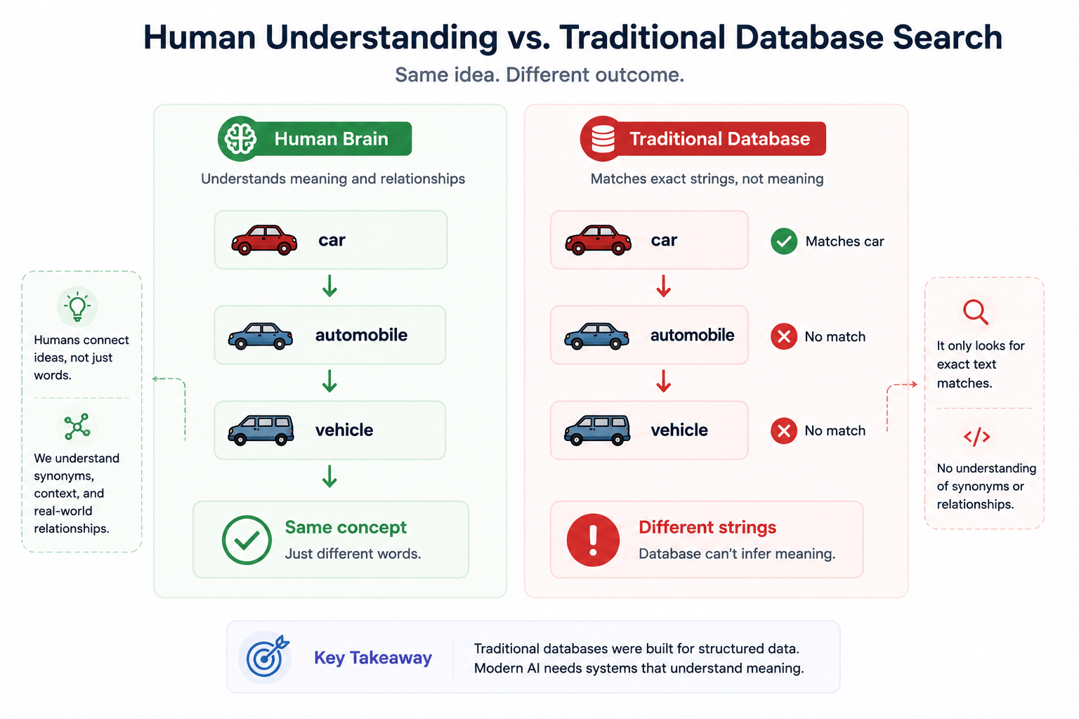
This difference seems small until your application contains millions of documents.
Now imagine you're building an AI assistant for a hospital. A doctor searches for "heart attack treatment," but every medical document uses the clinical term "myocardial infarction." A traditional keyword search may completely miss the most relevant documents—not because they don't exist, but because the wording is different.
The same problem appears everywhere.
A customer asks for “cancel my subscription” the documentation says “terminate recurring billing”. An engineer searches for “login bug” the issue tracker says ”authentication failure”. The ideas are identical. The words are not.
Traditional search systems don't understand this distinction because they don't search ideas. They search text.
Modern search engines became much smarter over time.
Instead of simply matching words, algorithms like BM25 rank documents based on how important each term is within a document and across an entire collection.
This dramatically improved search quality.
But it still depends on matching words.
If two documents describe the same idea using completely different vocabulary, lexical search can still fail.
This isn't a flaw in SQL.
It isn't a flaw in Elasticsearch.
And it certainly isn't a flaw in BM25.
They're solving the problem they were designed to solve: finding documents that contain matching terms.
Modern AI, however, asks a completely different question.
Instead of asking:
Which documents contain these words?
And for decades, they've answered that question remarkably well. Banking systems, search engines, e-commerce websites, and enterprise applications still rely on these technologies because matching structured data and keywords is exactly what they were built to do.
Modern AI, however, asks an entirely different question.
Which documents express this meaning?
That subtle shift changes everything.
Instead of comparing characters in a string, AI systems need to compare ideas. Instead of searching for exact words, they need to recognize that car, automobile, and vehicle often describe the same concept—even when none of those words appear together.
Traditional databases were never designed to understand relationships like these.
Not because they're poorly designed.
Because they were solving a different problem.
The challenge is that computers don't naturally understand meaning. They only understand numbers.
So if we want a machine to search ideas instead of words, we first need to answer a much deeper question:
How do you convert language into mathematics?
That question led to one of the most important breakthroughs in modern AI: Embeddings.
Join the frequency
Subscribe to our newsletter for the latest updates.
2. The Birth of Embeddings: Turning Meaning into Coordinates6 min read
Imagine opening Google Maps and searching for Paris. Within milliseconds, the application knows exactly where Paris is. It doesn't need a photograph of the city or a written description of its history. Instead, Paris is represented by a set of coordinates that uniquely identify its location on Earth. Those coordinates don't describe what Paris looks like—they simply tell us where it exists on a map.
Now imagine replacing cities with ideas.
Suppose someone says the word car. Without consciously thinking about it, your brain immediately connects it to automobile, vehicle, SUV, truck, and dozens of related concepts. If someone instead says banana, your mind instinctively places that idea somewhere completely different. Somehow, your brain behaves as though every concept occupies a position inside an invisible mental map where similar ideas naturally live close together while unrelated ideas drift farther apart.
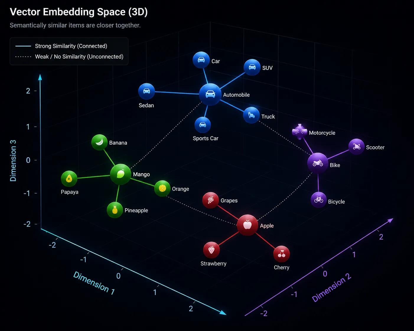
No one ever handed you this map.
You built it throughout your life by reading, listening, observing, and experiencing the world. Every conversation, every book, every article, and every memory subtly adjusted where ideas belonged inside your understanding of language.
Modern language models learn something remarkably similar.
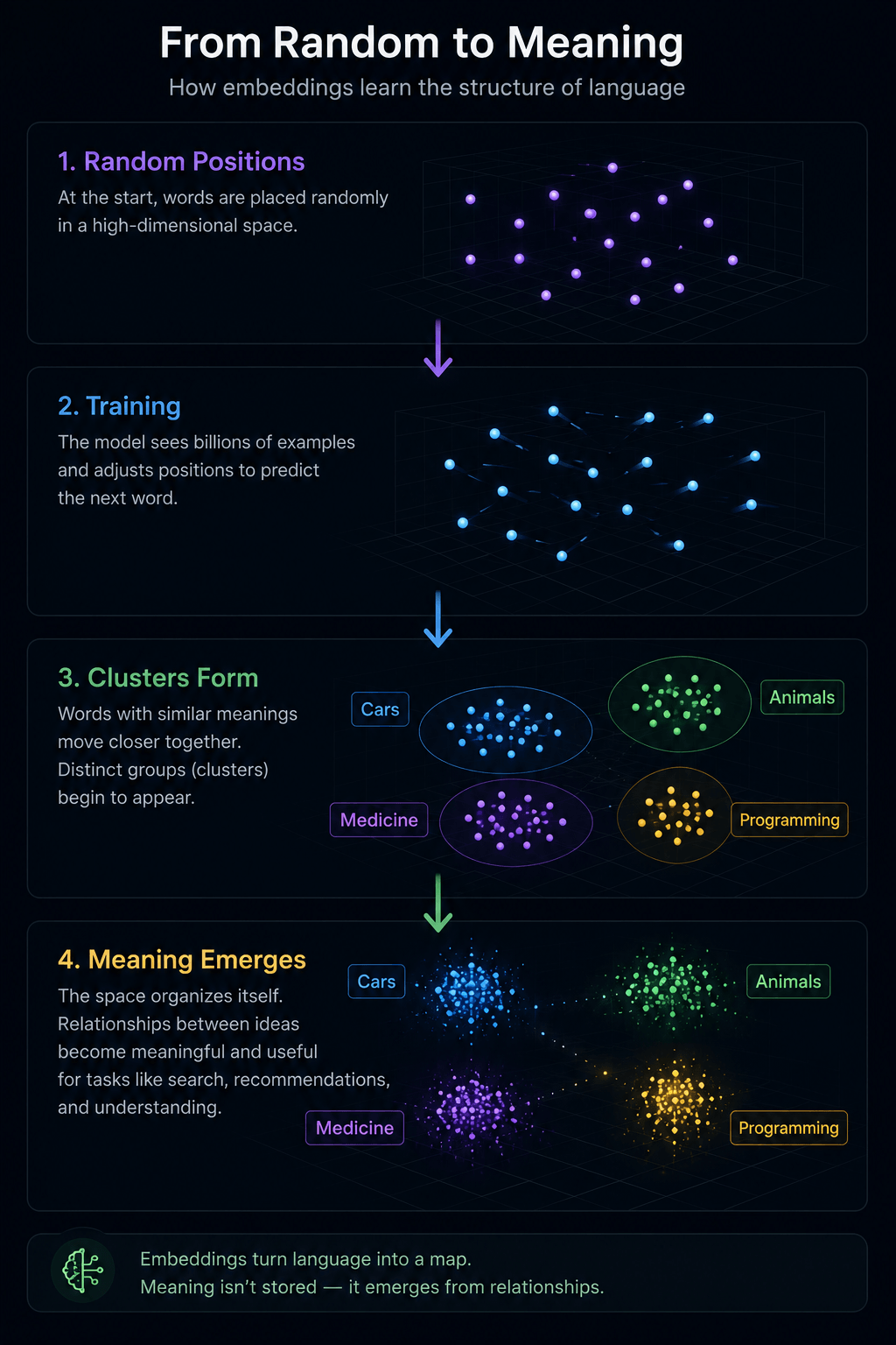
Instead of memorizing dictionary definitions or storing lists of synonyms, they gradually organize language into a mathematical landscape. During training, the model repeatedly encounters billions of words appearing together in different contexts. Words and phrases that frequently appear in similar situations slowly migrate toward one another, while concepts that rarely share context naturally separate. Over time, the model constructs a representation of language where meaning emerges from position rather than from explicit rules.
This is one of the most profound shifts in modern artificial intelligence.
Machines don't learn that car means automobile because someone programmed that relationship. They learn it because, across billions of examples, both words appear in remarkably similar contexts. News articles, technical documents, conversations, research papers, and books all reinforce the same statistical relationships until the model begins organizing language into neighborhoods of meaning.
The result is not a dictionary.
Think of an embedding as a GPS location for an idea.
Google Maps doesn't store Paris by describing its streets.
It stores where Paris exists.
Embedding models do the same thing for language.
They don't store "meaning."
They store where meaning lives.
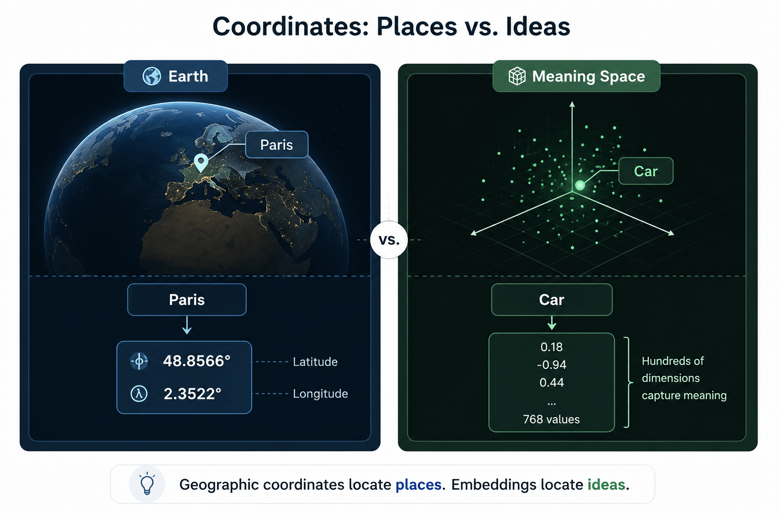
Instead of two coordinates, modern embedding models often describe every word, sentence, paragraph, or document using hundreds or even thousands of numerical coordinates. You don't need to visualize all of these dimensions individually. The important idea is much simpler: every additional coordinate gives the model another way to distinguish meaning. Just as adding altitude creates a richer representation of the physical world than a flat map alone, additional dimensions allow language models to capture increasingly subtle relationships between ideas.
These coordinates are called embeddings.
An embedding is simply the location of an idea inside this mathematical landscape.
Which two words should live closest together?
Car
Automobile
Banana
Pause for two seconds before continuing.
Notice what this definition deliberately avoids. An embedding is not the meaning itself. It is not a definition, a summary, or a collection of keywords. It is an address. Just as geographic coordinates tell us where Paris exists on Earth, an embedding tells us where a concept exists inside a space of meaning. Two ideas that occupy nearby locations are usually related, while ideas that appear far apart tend to describe completely different concepts.
But where do these coordinates come from?
Nobody manually assigns them.
from sentence_transformers import SentenceTransformer

model = SentenceTransformer("all-MiniLM-L6-v2")

embedding = model.encode(
    "Artificial intelligence is changing search."
)

print(len(embedding))384This sentence has now become 384 coordinates describing where its meaning exists in semantic space.
This is why modern embedding models can recognize relationships they were never explicitly taught. They understand that doctor is related to hospital, programmer is related to software, and planet is related to solar system, not because someone encoded those facts by hand, but because the geometry of language naturally emerged during training.
Once every sentence, document, image, or piece of code can be represented as coordinates, something extraordinary becomes possible.
Common Misconception
Embeddings are often described as vectors.
That's mathematically correct.
But for intuition, it's more useful to think of them as coordinates on a map of meaning.
The mathematics comes later.
Searching for information is no longer a problem of comparing words.
It becomes a problem of comparing locations.
And once information becomes location, the next question almost asks itself:
If every document has coordinates, how do we determine which ones are closest to our query?
That question leads us directly to the mathematics of similarity search.
📚 WANT TO DIVE DEEPER?
Embeddings Explained: How AI Converts Language into Mathematics
3. Similarity Search: Finding Meaning Through Distance8 min read
Imagine you've just converted every document in your database into coordinates. Your research papers, customer support articles, source code, emails, and documentation all now exist as points inside a massive mathematical landscape.
A user asks:
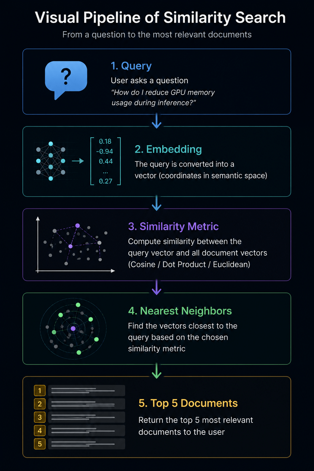
"How do I reduce GPU memory usage during inference?"
That question is also converted into coordinates using the same embedding model. Instead of searching through millions of documents word by word, the system places the query onto the same map.
Now the problem becomes surprisingly simple.
The database doesn't ask:
"Which documents contain these words?"
Instead, it asks:
"Which documents are closest to this point?"
Everything that follows in a modern vector database is built around answering that single question as efficiently as possible.
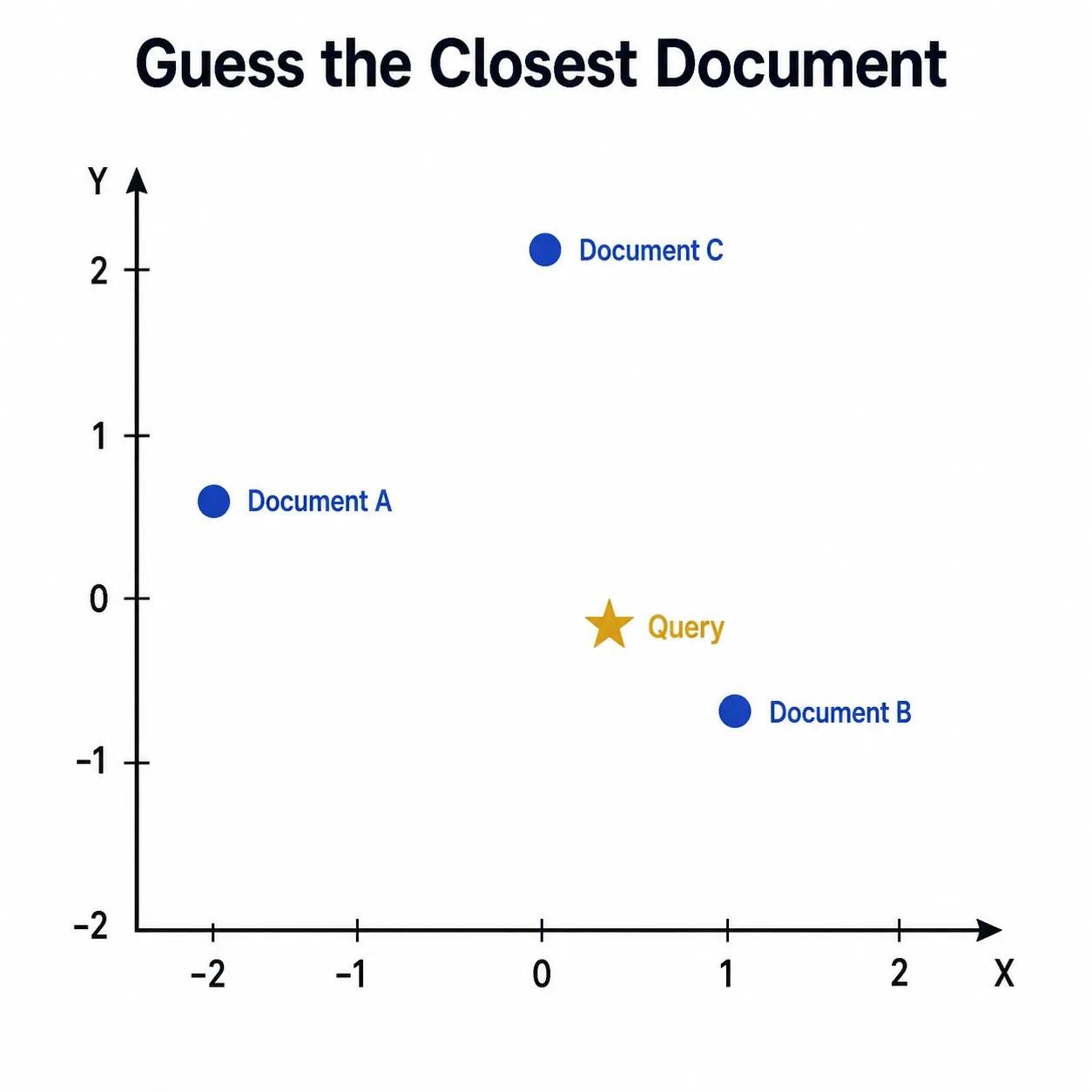
Without calculating anything, which document do you think is most similar to the query?
Humans solve this kind of problem instinctively. If someone asks which café is closest to your house, you don't compare every café in the city. You estimate which locations are nearest based on distance.
Vector databases do exactly the same thing.
The only difference is that instead of measuring physical distance between cities, they measure mathematical distance between ideas.
But this immediately raises another question.
How should we measure that distance?
Surprisingly, there isn't just one answer.
Different applications use different definitions of "close," and each one changes how similarity is calculated.
Measuring Similarity
If two cities are only one kilometer apart, we naturally consider them close together.
Ideas work similarly, but in high-dimensional mathematical space we need formulas to measure closeness.
The three most common approaches are Euclidean Distance, Cosine Similarity, and Dot Product. While they often produce similar results, they answer subtly different questions and are suited for different types of embedding models.
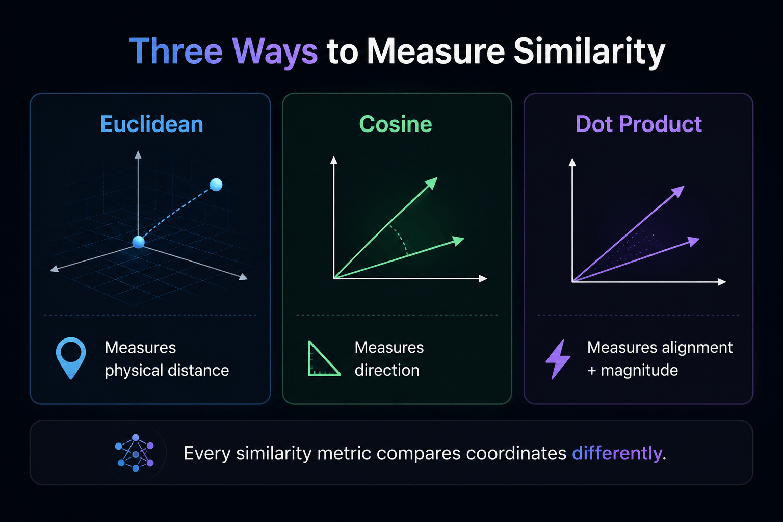
Euclidean Distance: The Straight-Line Answer
Euclidean distance is the most intuitive because it matches how we think about the physical world.
Imagine standing in a park.
One friend is standing five meters away.
Another is standing twenty meters away.
Without any calculations, you know which person is closer.
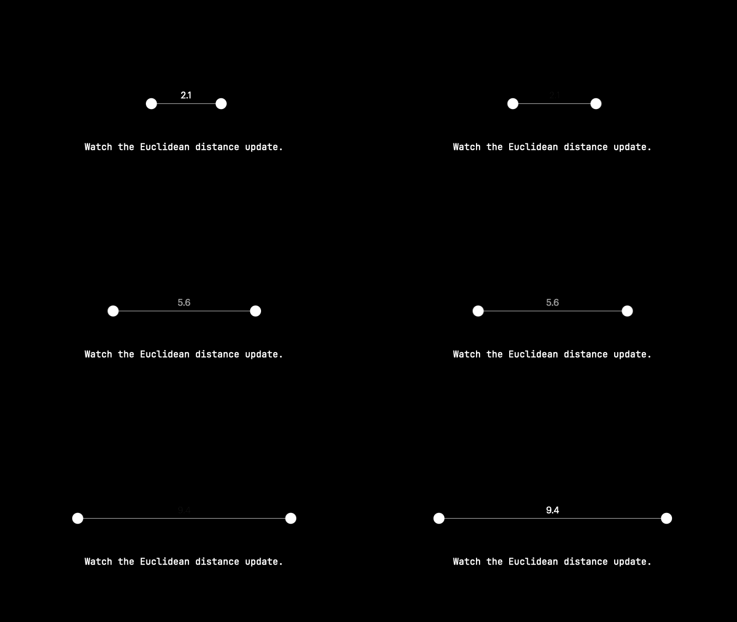
Euclidean distance asks exactly the same question inside an embedding space:
"What is the shortest straight-line distance between these two points?"
If the distance is small, the ideas are considered similar.
If the distance is large, they are considered different.
This approach is easy to understand and works well for many applications, but modern language models often care less about absolute distance and more about whether two ideas point in the same semantic direction.
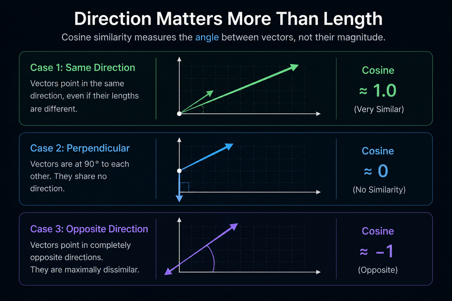
Cosine Similarity: Comparing Direction Instead of Distance
Now imagine two arrows.
One is short.
One is long.
Both point in exactly the same direction.
Are they describing the same idea?
In many language models, the answer is yes.
Cosine similarity ignores how long the arrows are and focuses almost entirely on where they point. If two embeddings have nearly the same direction, cosine similarity considers them highly related, even if their magnitudes differ significantly.
This turns out to be an incredibly useful property for semantic search because meaning is often captured more by direction than by absolute length.
As a result, cosine similarity has become one of the most widely used metrics in modern embedding systems.
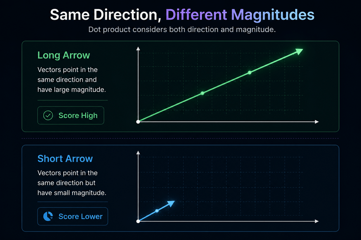
Dot Product: Similar Direction, Strong Confidence
Dot product is closely related to cosine similarity but also considers the magnitude of the embeddings.
Imagine two arrows pointing in the same direction.
If both arrows are long, the dot product becomes larger.
If one arrow is much shorter, the score decreases.
This additional information can be valuable because some embedding models intentionally encode confidence or importance through vector magnitude.
For this reason, several modern retrieval systems use dot product instead of cosine similarity, particularly when working with embedding models trained for Maximum Inner Product Search (MIPS).
Which One Is Best?
This is one of the most common questions asked by developers.
The answer is:
It depends on the embedding model.
Some models are trained assuming cosine similarity.
Others optimize for dot product.
Some normalize embeddings, making Euclidean distance and cosine similarity produce nearly identical rankings.
The important lesson isn't to memorize formulas.
It's to understand that similarity is not a universal concept.
Every embedding model defines "close" slightly differently.
Code Example: Calculating Similarity with NumPy
Once embeddings are represented as arrays of numbers, calculating similarity becomes surprisingly straightforward.
import numpy as np

car = np.array([0.42, 0.18, -0.91])
automobile = np.array([0.39, 0.16, -0.89])

cosine = np.dot(car, automobile) / (
    np.linalg.norm(car) * np.linalg.norm(automobile)
)

print(cosine)0.998A score close to 1 indicates that the two embeddings are pointing in nearly the same direction, suggesting they represent highly similar meanings.
Similarity is not intelligence.
A vector database does not "understand" language in the way humans do. It performs mathematical comparisons between coordinates produced by an embedding model. The intelligence comes from how those embeddings were learned, not from the database itself.
Code Example: FAISS
Finding the closest document becomes even more efficient using libraries like FAISS.
import faiss
import numpy as np

index = faiss.IndexFlatIP(384)

index.add(document_embeddings)

scores, indices = index.search(
    query_embedding,
    k=5
)
In just a few lines, FAISS searches thousands—or even millions—of embeddings and returns the nearest neighbors to the query.
As elegant as this approach is, one practical question remains.
Finding the closest point among ten documents is easy.
Finding the closest point among ten million documents is something entirely different.
Modern AI systems can't afford to compare every query against every embedding one by one. At production scale, that would be far too slow for real-time search, recommendations, or Retrieval-Augmented Generation (RAG).
Clearly, we need something more than just embeddings and similarity metrics.
We need a system that can store, organize, filter, and search billions of embeddings efficiently while returning results in milliseconds.
That system is called a vector database.
And understanding what it actually does is the next piece of the puzzle.
🛠️ Book Worth Reading

Introduction to Information Retrieval
If you'd like to understand the foundations of search engines—including BM25, ranking, indexing, and retrieval theory—Introduction to Information Retrieval remains one of the classic texts in the field.
Try Introduction to Information Retrieval4. So What Is a Vector Database?8 min read
What Is a Vector Database
A vector database is a database designed to store, organize, index, filter, and search vector embeddings efficiently. It enables semantic search by retrieving the most similar vectors to a query, even across millions or billions of documents, while supporting metadata filtering, updates, and real-time retrieval.
The previous sections answered three fundamental questions.
First, we discovered why traditional keyword search struggles to understand meaning. Then we learned how language models convert words into coordinates through embeddings. Finally, we explored how similarity metrics allow computers to compare those coordinates mathematically.
But one obvious question still remains.
If every document becomes an embedding, where do all of those embeddings actually live?
Modern AI systems aren't comparing vectors stored inside a spreadsheet or loading millions of embeddings into memory every time a user asks a question. They need a system that can permanently store these representations, retrieve them in milliseconds, update them as new information arrives, and filter them using metadata such as author, date, language, or document type.
That system is called a vector database.
Unlike traditional databases, which primarily organize rows and columns, a vector database is optimized around one central task: storing embeddings and retrieving the most semantically similar ones as quickly as possible. Everything else—indexes, metadata, storage engines, replication, and filtering—exists to make that retrieval efficient at scale.
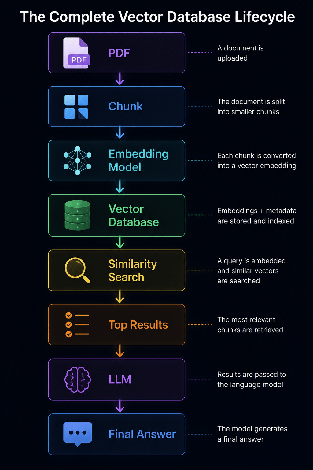
Every modern Retrieval-Augmented Generation (RAG) system follows this general pipeline. The vector database sits between embeddings and the language model, retrieving relevant context before the LLM generates a response.
Once you see the entire pipeline, the role of a vector database becomes much easier to understand.
Imagine uploading a 500-page PDF into an AI assistant.
The language model doesn't memorize that document.
Instead, the document is broken into smaller chunks—typically paragraphs or sections that can fit comfortably inside an embedding model's context window. Each chunk is then converted into an embedding, transforming human language into coordinates that represent meaning.
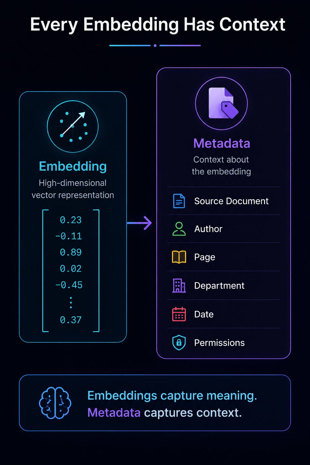
These embeddings, along with useful metadata such as the source document, page number, title, author, or publication date, are stored inside the vector database.
Later, when someone asks a question, the exact same embedding model converts the query into coordinates. Instead of searching the original text directly, the database searches for embeddings located nearest to the query in semantic space. The matching document chunks are returned to the application, which then passes them to the language model as context before generating the final response.
The LLM never searched the PDF itself.
The vector database did.
Think Through the Pipeline
Imagine you've uploaded a textbook on machine learning.
Now ask yourself:
"What happens first?"
Arrange these steps into the correct order:
- Document is chunked
- Query arrives
- Embeddings are created
- Similar documents are retrieved
- LLM generates an answer
Storing More Than Just Embeddings
One common misconception is that vector databases only store embeddings.
In practice, they store much more.
Every embedding is usually accompanied by metadata that describes the original content. This metadata doesn't influence semantic meaning directly, but it allows applications to filter results before or after similarity search.
For example, an enterprise knowledge base might store information like:
When someone searches for "parental leave policy," the database can first limit the search to HR documents written in English before performing similarity search on the remaining embeddings.
Without metadata, semantic search would often return relevant—but unusable—results.
CRUD Still Exists
Although vector databases introduce new ways of searching, they haven't abandoned traditional database operations.
Applications still need to create, update, delete, and retrieve records as information changes over time.
Imagine a company updating its employee handbook.
The old document shouldn't remain searchable forever.
Instead, the application removes the outdated embeddings, generates new ones from the revised document, and inserts them back into the database. The process feels familiar to anyone who has worked with relational databases—only the stored data happens to be embeddings rather than rows of structured values.
This means vector databases support many of the same operations developers already expect:
- Create new embeddings when new documents arrive.
- Read embeddings during similarity search.
- Update metadata or replace outdated embeddings.
- Delete documents that should no longer appear in search results.
Semantic search may be new, but database fundamentals still apply.
from pinecone import Pinecone

pc = Pinecone(api_key="YOUR_API_KEY")

index = pc.Index("knowledge-base")

index.upsert([
    {
        "id": "doc-101",
        "values": embedding,
        "metadata": {
            "title": "Employee Handbook",
            "department": "HR"
        }
    }
])Key Insight
This example inserts a document embedding together with searchable metadata. Later, the metadata can be used to filter results before similarity search.
Filtering Before Searching
One of the biggest advantages of vector databases is that semantic similarity doesn't have to search everything.
Suppose you're building a multilingual AI assistant.
A user asks a question in French.
Even if the database contains millions of English documents, there's no reason to search them.
Instead, the application can first filter documents where:
language = "French"Only then does similarity search begin.
This combination of metadata filtering and semantic retrieval makes vector databases both faster and more accurate than searching every embedding indiscriminately.
Searching at Scale
Everything we've discussed so far works perfectly for hundreds of documents.
Real production systems are very different.
GitHub Copilot indexes billions of lines of code.
Enterprise search systems index decades of documentation.
Scientific databases contain millions of research papers.
Medical retrieval systems store enormous collections of clinical literature.
Searching through every embedding individually would quickly become impossible.
The challenge is no longer understanding meaning.
The challenge is finding nearby embeddings quickly enough that users never notice the search happening.
Comparison
| Traditional Database | Vector Database |
|---|---|
▸Stores structured rows | ▸Stores embeddings |
▸Retrieves exact matches | ▸Retrieves similar meaning |
▸Optimized for transactions | ▸Optimized for nearest-neighbor search |
▸Primary key lookups | ▸Semantic retrieval |
Code Example – pgvector
One of the most interesting aspects of vector search is that you don't always need a dedicated vector database.
Extensions like pgvector allow PostgreSQL to store embeddings directly alongside traditional relational data.
CREATE TABLE documents (
    id SERIAL PRIMARY KEY,
    content TEXT,
    embedding VECTOR(768)
);
This makes it possible to combine SQL queries with semantic search, giving developers the best of both worlds for many applications.
A vector database is not a language model.
It doesn't generate answers.
It doesn't understand language on its own.
Its job is to store embeddings efficiently, retrieve the nearest neighbors, and return them to the application or language model.
The intelligence comes from the embedding model and the LLM—not from the database itself.
Everything now fits together.
Documents become chunks.
Chunks become embeddings.
Embeddings are stored inside a vector database.
Queries become embeddings.
Similarity search retrieves the nearest neighbors.
The language model receives those retrieved results as context before generating a final answer.
At this point, we understand each individual component.
But modern AI systems don't use these components in isolation.
They work together as part of a much larger retrieval pipeline.
When you upload a PDF to ChatGPT, GitHub Copilot searches your codebase, or an enterprise AI assistant answers questions about internal documentation, dozens of operations happen behind the scenes before the language model generates its first token.
The vector database is only one piece of that system.
So before we open the database itself and explore its internal architecture, let's step back and look at the complete picture.
What actually happens when you ask ChatGPT a question about your company's PDF?
5. What actually happens when you ask ChatGPT a question about your company's PDF?9 min read
Imagine your company has accumulated ten years of documentation.
Employee handbooks, engineering specifications, API documentation, meeting notes, research papers, design documents, contracts, incident reports, and thousands of internal knowledge base articles are scattered across different systems. Somewhere inside those documents lies the answer to your question—but no language model has memorized any of it.
Now imagine asking an AI assistant:
"What changed in our API authentication system after version 4?"
The response arrives in just a few seconds.
How?
Did the language model search every PDF?
Did it memorize every document?
Or did it somehow connect to your company's file system?
The answer is none of those.
Behind the scenes, an entire retrieval pipeline begins working long before the language model generates its first word. Every component has a specific responsibility, and understanding this pipeline explains not only how Retrieval-Augmented Generation (RAG) works, but also why vector databases have become one of the most important pieces of modern AI infrastructure.
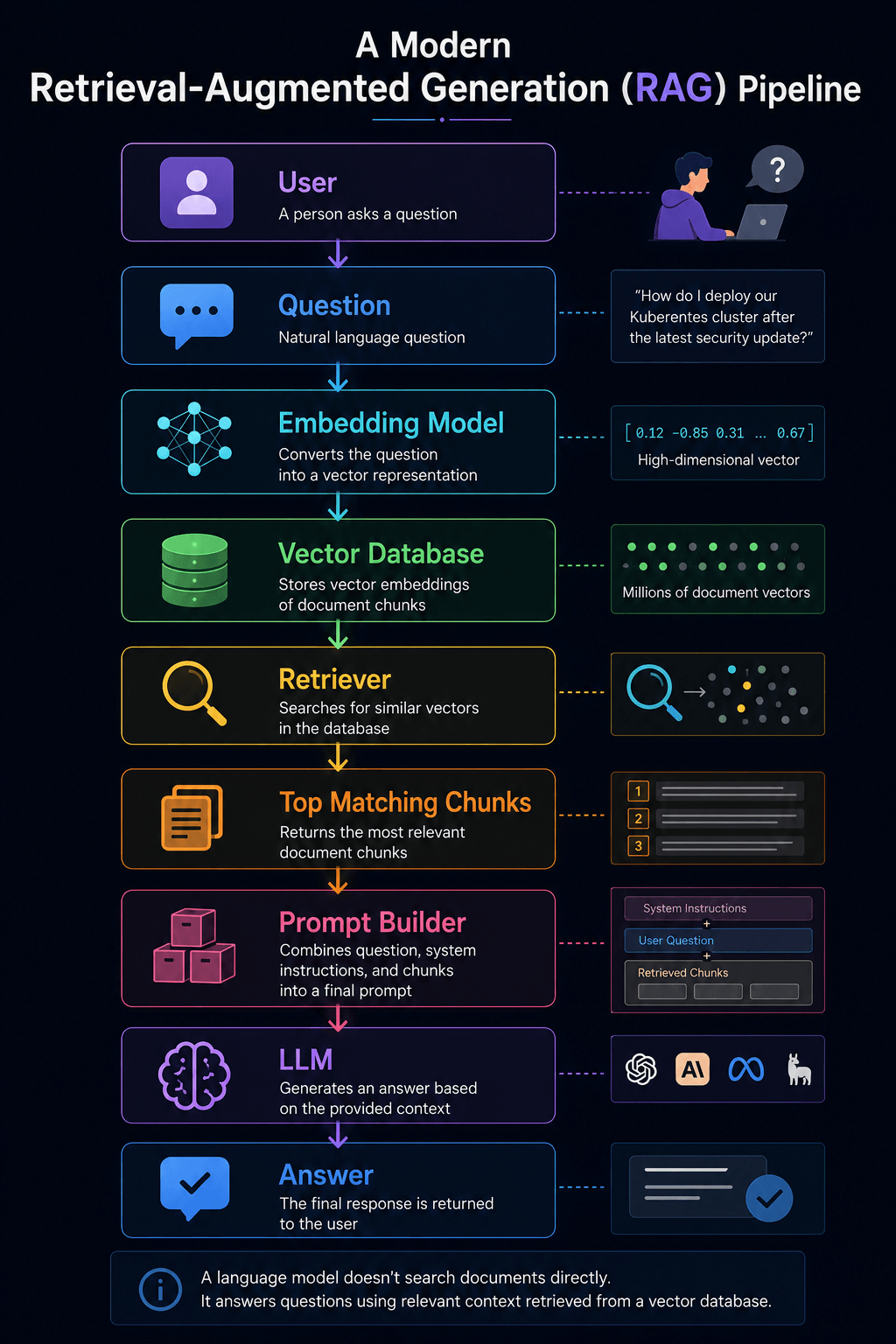
The first thing to notice is that the language model appears almost at the end of the pipeline—not at the beginning.
That surprises many people.
The language model isn't responsible for finding information. Its primary responsibility is generating natural language. Finding the right information belongs to an entirely different retrieval system.
Let's follow the journey one step at a time.
Step 1 — The User Asks a Question
Everything begins with a natural language query.
Suppose a software engineer asks:
"How do I deploy our Kubernetes cluster after the latest security update?"
To a human, this looks like an ordinary sentence.
To the retrieval system, it's simply the starting point of a search operation.
Before anything can be retrieved, the question itself must be transformed into an embedding using exactly the same embedding model that was used to process the company's documents.
Only then do the query and the documents exist inside the same semantic space.
What Should Be Embedded?
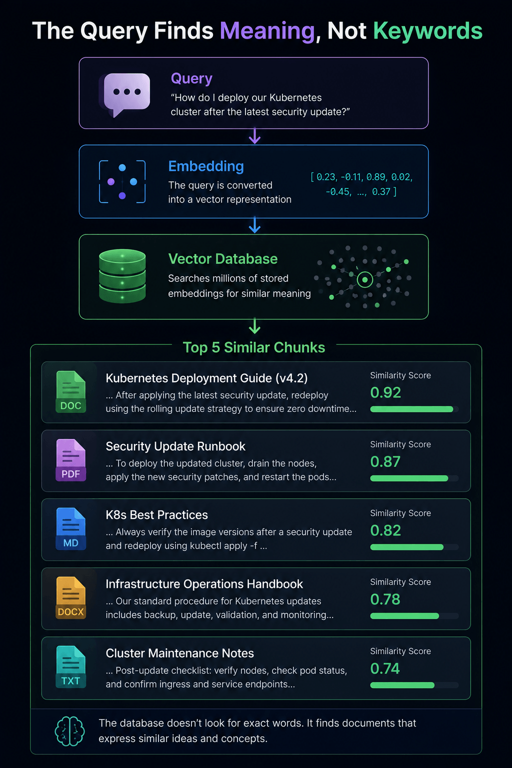
Step 2 — Searching the Vector Database
Once the question becomes coordinates, the vector database takes over.
Instead of scanning documents line by line, it searches through millions of stored embeddings looking for nearby points in semantic space. The retrieval system doesn't care whether the documents contain identical words. It only cares whether they express similar ideas.
If the engineer searches for "API authentication," the database may retrieve documents discussing OAuth tokens, JWT validation, or identity providers, even if the original wording is completely different.
This is the moment where semantic search replaces keyword search.
Step 3 — Retrieving Context
Notice something important.
The vector database does not return an answer.
It returns document chunks.
Those chunks might be paragraphs from an employee handbook, sections of API documentation, pieces of source code, or excerpts from technical specifications. Individually they are just fragments of information, but together they provide the evidence the language model needs to answer accurately.
This distinction is critical.
Vector databases retrieve.
Language models generate.
Confusing these two responsibilities is one of the most common misunderstandings in modern AI systems.
Mental Model
Think of the vector database as a librarian.
It finds the right books.
The language model is the author who reads those books and writes a clear answer.
Neither can replace the other.
Step 4 — Building the Prompt
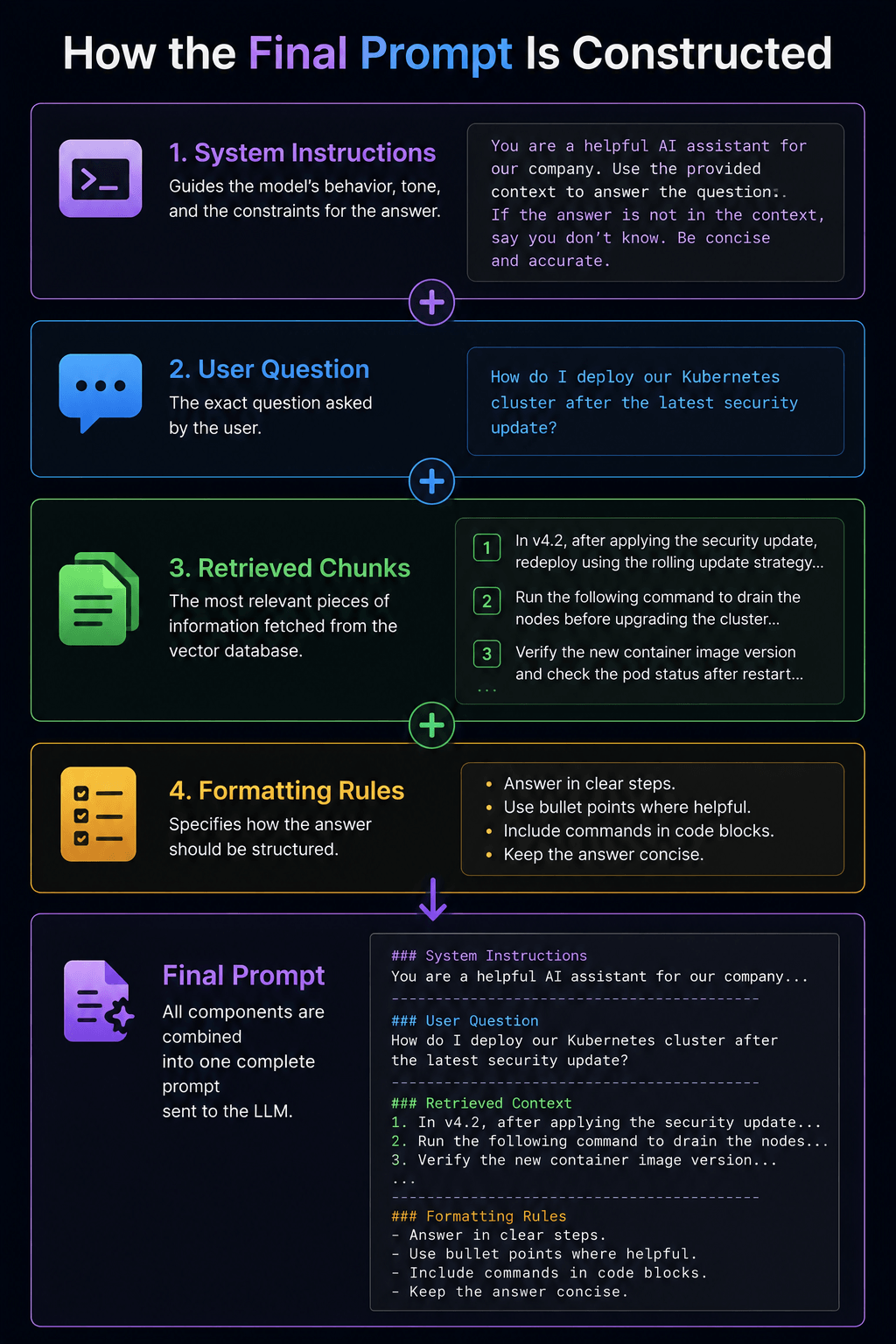
The retrieved document chunks are now combined with the user's original question.
Instead of asking the language model only:
"How do I deploy Kubernetes?"
the application sends something much richer.
It includes the user's question, the retrieved document excerpts, system instructions, formatting rules, and any additional context required for the task.
This entire package becomes the final prompt.
The language model now has the information it needs to answer accurately without relying solely on its training data.
Step 5 — The Language Model Generates the Answer
Only now does the language model begin generating text.
By this stage, the difficult work has already been completed.
The documents have been embedded.
The vector database has retrieved the relevant context.
The prompt has been assembled.
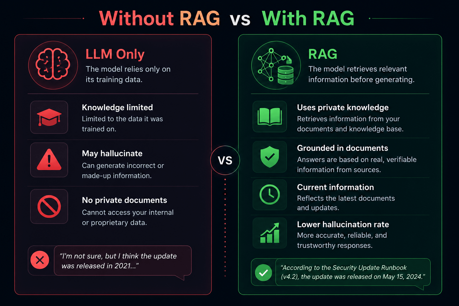
The language model simply reasons over the supplied information and produces a response grounded in the retrieved documents.
This is why modern AI assistants can answer questions about information that never existed during their original training.
The knowledge wasn't memorized.
It was retrieved.
Step 6 — Where the Vector Database Fits
By now, the role of the vector database should feel much clearer.
It doesn't replace SQL.
It doesn't replace the language model.
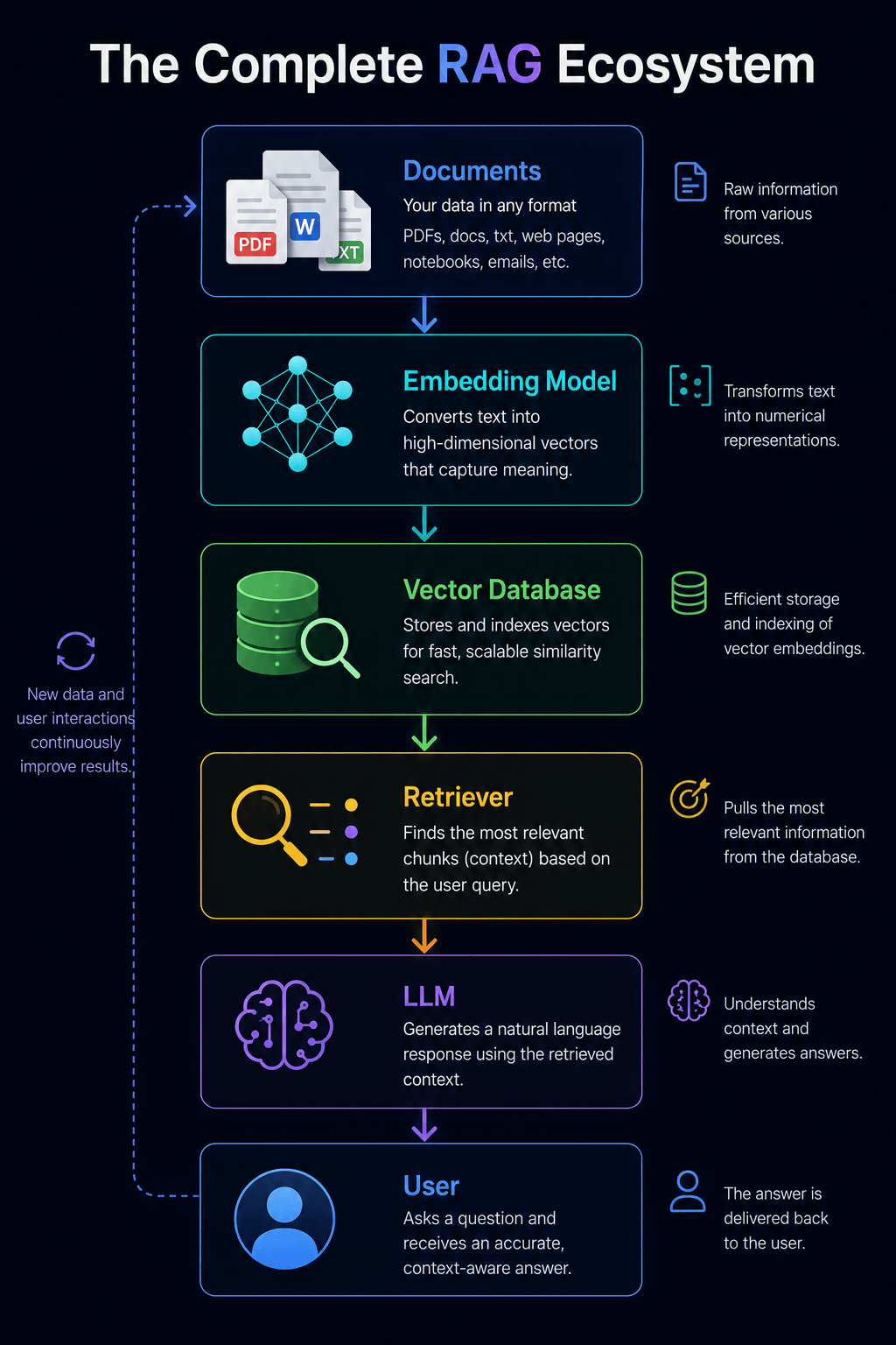
Instead, it becomes the bridge connecting stored knowledge with intelligent generation.
Without the vector database, the language model has no efficient way to search millions of documents.
Without the language model, retrieved documents remain unorganized fragments.
Together, they form a complete retrieval system.
Building This in Production
The architecture you've just seen isn't limited to research labs.
Thousands of production systems use a remarkably similar stack.
A typical deployment might include:
Notice that every layer can be replaced independently. You can swap the embedding model without changing the API, replace the vector database without modifying the frontend, or migrate from a hosted language model to a local model while preserving the rest of the architecture. This modularity is one of the reasons RAG systems have become so popular in production.
query = embed(user_question)

results = vector_db.search(
    query,
    top_k=5
)

prompt = build_prompt(
    user_question,
    results
)

answer = llm.generate(prompt)
Even production RAG systems follow this same logical sequence, although each step is usually implemented with much greater sophistication.
Drag them into the correct order.
Production Tools
If you're building a RAG application yourself, these tools are widely adopted and well supported:
🛠️ Tools Worth Exploring
Pinecone
A managed vector database for storing and searching embeddings efficiently.
Try PineconeRunpod
A cloud platform that provides on-demand GPU infrastructure for AI development, training, and inference.
Try RunpodRAG is not a model
Retrieval-Augmented Generation is a system architecture. It combines embeddings, vector databases, retrieval, prompt construction, and a language model into a single pipeline. No single component is "RAG" on its own.
The pipeline is now complete.
We know how documents become embeddings, how embeddings are stored, how relevant information is retrieved, and how a language model transforms that retrieved context into an answer.
One question remains.
When the vector database receives a query, what actually happens inside it?
How are millions of embeddings stored, indexed, filtered, replicated, and searched fast enough to respond in milliseconds?
To answer that, we need to open the database itself and examine the engineering hidden beneath the API. That is the focus of the next chapter: Inside a Vector Database.
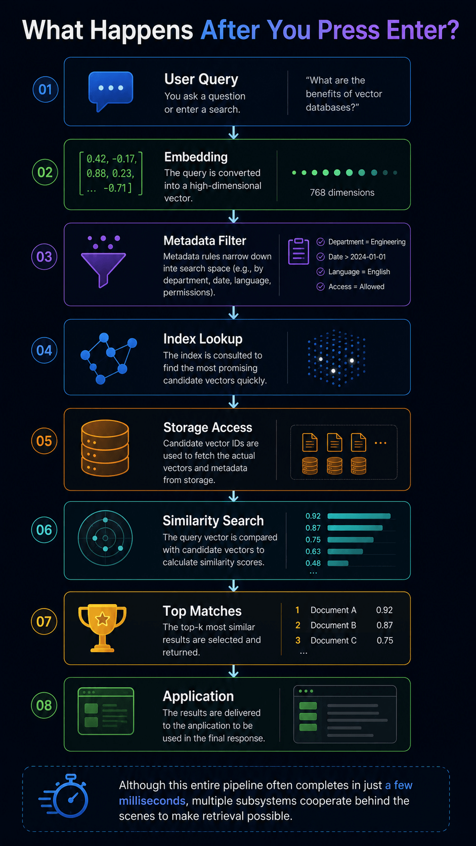
6. Inside a Vector Database: What Happens After You Press Enter?8 min read
The previous chapter followed the journey of your question through an entire Retrieval-Augmented Generation (RAG) pipeline. By the time the query reached the vector database, it had already been transformed into an embedding, and the database's job was clear: find the most relevant pieces of information as quickly as possible.
From the outside, this process looks almost effortless. A question is submitted, a few milliseconds pass, and the application receives the document chunks it needs.
But inside the database, something far more sophisticated is happening.
Imagine pausing time at the exact moment you press Enter.
Your query has just become an embedding.
It is now approaching a database containing millions—or perhaps billions—of other embeddings.
What happens next?
To answer that question, we need to open the database itself.
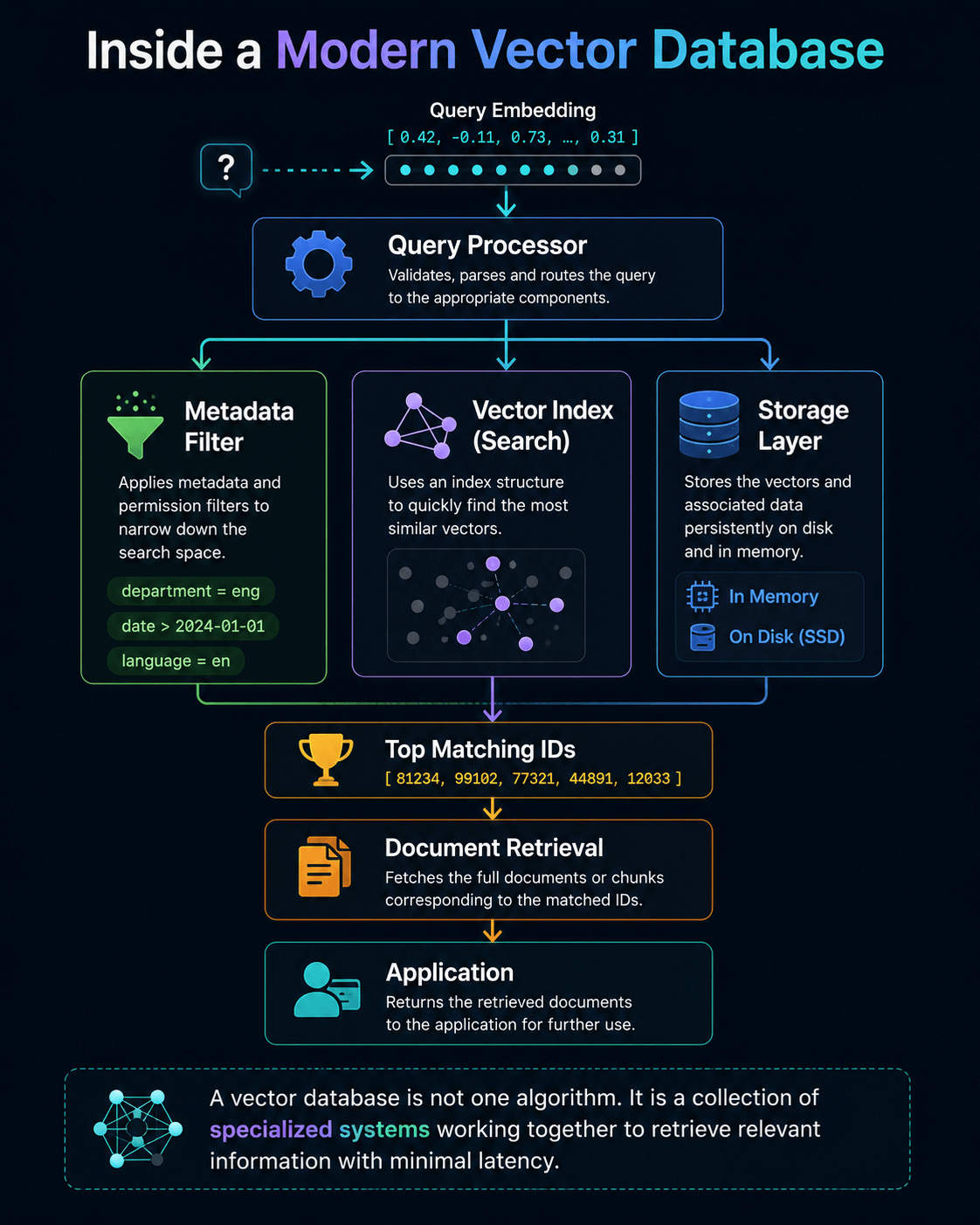
The first thing to understand is that a vector database is much more than a collection of embeddings.
If you were to open its storage engine, you wouldn't find millions of vectors arranged neatly in a single file waiting to be searched. Instead, you would discover multiple specialized components, each responsible for solving a different problem.
Some components decide where embeddings should be stored.
Others manage metadata.
Others organize indexes that make retrieval fast.
Others replicate data across machines to prevent failures.
Still others compress embeddings to reduce memory usage.
All of these systems cooperate every time a query arrives.
The similarity search we explored earlier is only one small part of the overall process.
Storage: Where Do Embeddings Actually Live?
After an embedding is generated, it has to be stored somewhere permanently.
During development, a few thousand vectors can comfortably fit inside memory.
Production systems are very different.
A customer support platform may index millions of conversations.
A code search engine may contain billions of source code embeddings.
Scientific search engines routinely process tens of millions of research papers.
The database therefore has to balance two competing goals.
It must retrieve vectors quickly while also storing enormous amounts of information efficiently.
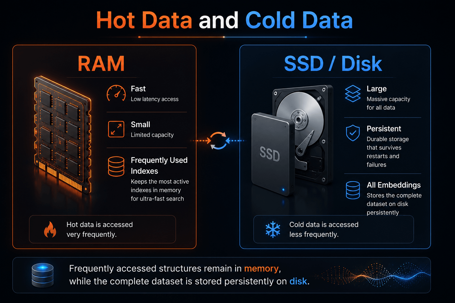
For this reason, modern vector databases typically divide storage into multiple layers. Frequently accessed indexes remain in memory for speed, while larger datasets are stored on disk and loaded only when necessary.
This approach is similar to how operating systems rely on RAM for active data while using SSDs or hard drives for long-term storage. The difference is that vector databases must optimize this process specifically for similarity search rather than general file access.
Metadata: Meaning Needs Context
Embeddings capture meaning.
They do not capture context.
Suppose two engineering documents discuss authentication systems.
One belongs to the mobile application.
The other belongs to the backend infrastructure.
Semantically, both documents may be very similar.
Without additional information, the database cannot distinguish between them.
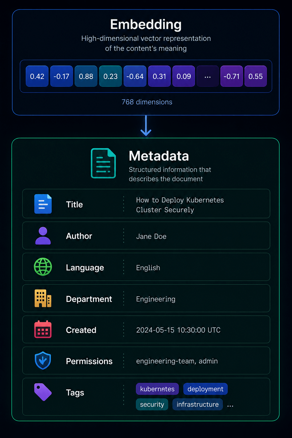
This is why vector databases store metadata alongside every embedding.
Metadata describes properties of the original document rather than its meaning.
It may include the document title, author, department, language, publication date, access permissions, or any other information the application needs during retrieval.
When a user searches only within engineering documentation published during the last six months, the database first uses metadata to reduce the search space before semantic retrieval even begins.
The result is both faster and more accurate.
Filtering Before Searching
Metadata becomes even more valuable when the database contains millions of embeddings.
Imagine searching every document in an enterprise knowledge base when you only have permission to access one department.
Not only would that waste computational resources, it could also expose confidential information.
Instead, the retrieval engine first filters documents according to metadata rules.
Only the remaining embeddings participate in similarity search.
This dramatically reduces the amount of work the database must perform while ensuring the retrieved information satisfies application requirements.
Most production AI systems combine metadata filtering and semantic retrieval for exactly this reason.
Indexes: Organizing the Search Space
Imagine walking into a library containing twenty million books with no shelves, no catalog, and no organization.
Finding a single book would require examining every book one by one.
A vector database faces the same challenge.
Embeddings cannot simply be stored in one enormous collection.
They must be organized so nearby vectors can be found quickly.
This organization is called an index.
An index is not the data itself.
It is a specialized structure that tells the database where it should search.
Just as a book index points readers toward relevant pages instead of forcing them to read the entire book, a vector index dramatically reduces the amount of work required during retrieval.
In the next chapter we will explore exactly how indexes such as HNSW, IVF, and DiskANN accomplish this.
For now, the important idea is much simpler.
The index is what transforms an enormous collection of embeddings into something searchable.
Think of an index as a map, not a storage device.
Embeddings contain the information.
Indexes tell the database where to look.
Compression: Fitting Billions of Embeddings Into Memory
A modern embedding may contain hundreds or thousands of numerical coordinates.
Now multiply that by one billion documents.
The amount of memory required quickly becomes enormous.
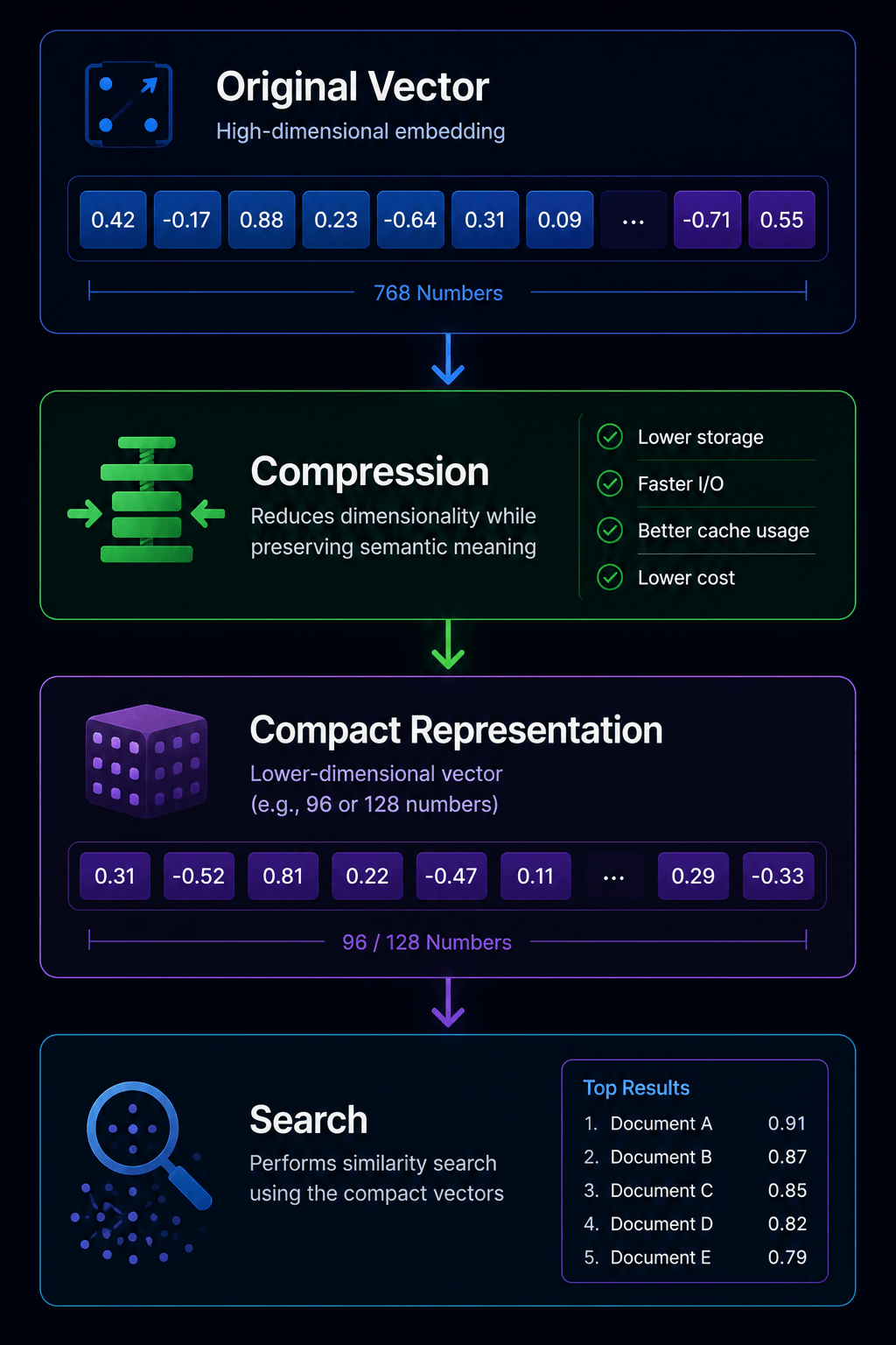
Rather than storing every embedding in its original form, many vector databases compress vectors while preserving as much semantic information as possible.
Compression reduces storage costs, improves cache efficiency, and allows larger datasets to fit inside memory.
The challenge is balancing storage savings against retrieval accuracy.
Compress too aggressively, and nearby embeddings may no longer remain nearby.
Compress too little, and infrastructure costs increase dramatically.
Finding the right balance is one of the key engineering decisions behind large-scale vector search systems.
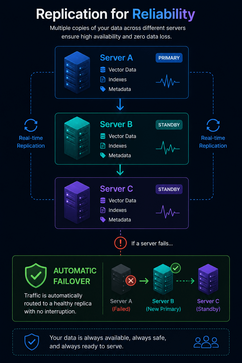
Replication: Preparing for Failure
Imagine an AI assistant serving millions of users every day.
What happens if one server suddenly crashes?
Without replication, every embedding stored on that machine becomes temporarily unavailable.
Modern vector databases avoid this problem by maintaining multiple copies of important data across different machines or availability zones.
If one server fails, another immediately continues serving requests.
Replication is not primarily about speed.
It is about reliability.
Users should never notice that hardware has failed.
Large production deployments therefore replicate indexes, metadata, and stored embeddings to eliminate single points of failure.
Putting Everything Together
By now, the internal architecture should feel much less mysterious.
A vector database is not simply storing embeddings.
It is simultaneously managing persistent storage, metadata, filtering rules, indexes, compression strategies, replication, and retrieval.
Every query passes through these components before the application receives its results.
Each layer exists because modern AI systems must balance speed, scalability, reliability, and cost.
At this point, we understand what a vector database stores and how its internal components cooperate.
But we have deliberately avoided one crucial question.
How does the index itself find nearby embeddings without comparing the query against every vector in the database?
That challenge lies at the heart of modern vector search.
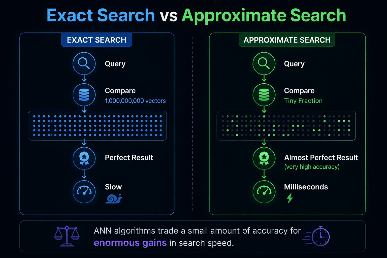
The answer is a family of algorithms collectively known as Approximate Nearest Neighbor (ANN) algorithms—techniques that allow databases to search billions of vectors in milliseconds while sacrificing only a tiny amount of accuracy.
The next chapter explores those algorithms in depth, beginning with the simplest possible approach: comparing every vector one by one, and why that quickly becomes impractical at scale.
🛠️ Want to understand why modern databases are designed this way?

Designing Data-Intensive Applications
Designing Data-Intensive Applications by Martin Kleppmann is one of the best books on distributed systems, storage engines, replication, indexing, and large-scale data architecture. Recommended for: Backend engineers, infrastructure engineers, AI platform developers.
Try Designing Data-Intensive Applications7. How Can a Database Search One Billion Vectors in Milliseconds?10 min read
By now, we've built almost the entire retrieval pipeline.
A user's question becomes an embedding. The vector database stores millions of document embeddings. Similarity search determines which documents are closest to the query, and the language model generates an answer using those retrieved results.
One critical question still remains.
Suppose your vector database contains one billion embeddings.
How does it find the nearest neighbors in just a few milliseconds?
The obvious solution seems straightforward.
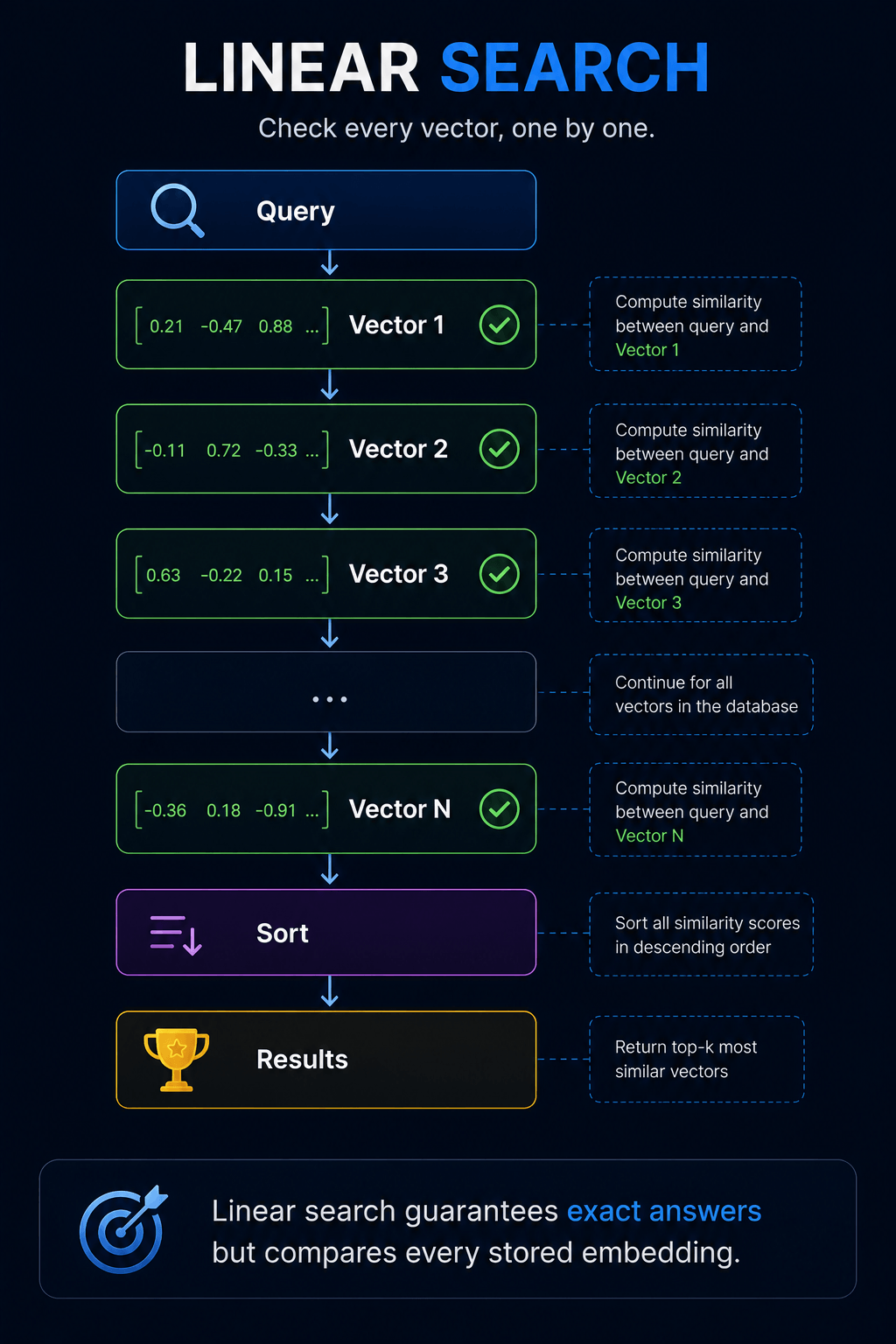
Compare the query with every embedding.
Measure the similarity.
Sort the results.
Return the closest vectors.
Mathematically, that works perfectly.
Practically, it becomes a disaster.
If every query required comparing itself against one billion vectors, even extremely fast hardware would struggle to deliver interactive response times. Every additional document would increase the amount of work the database must perform.
For a tiny dataset, this isn't a problem.
For production-scale AI systems, it quickly becomes impossible.
Modern vector databases solve this challenge using a family of techniques collectively known as Approximate Nearest Neighbor (ANN) algorithms.
Notice the word approximate.
These algorithms deliberately avoid checking every vector. Instead, they sacrifice a tiny amount of mathematical perfection in exchange for enormous improvements in speed.
Finding the exact nearest neighbor is sometimes less valuable than finding an almost identical neighbor one thousand times faster.
That tradeoff is what makes modern semantic search practical.
The Simplest Algorithm: Linear Search
Let's begin with the simplest possible solution.
Imagine you have only ten document embeddings.
When a query arrives, you calculate its similarity score against the first embedding, then the second, then the third, continuing until every document has been compared.
Finally, you sort the results and return the closest matches.
This approach is called linear search, sometimes referred to as brute-force search.
Conceptually, it's beautiful because it guarantees the mathematically correct answer. No approximations are involved, and no document is skipped.
For small datasets, linear search is often the best choice because it introduces almost no additional complexity.
The problem appears when the dataset begins to grow.
Searching one thousand embeddings is still manageable.
Searching one million is expensive.
Searching one billion for every user request becomes impractical.
The algorithm scales linearly with the number of stored vectors. Double the dataset, and you roughly double the work required for every search.
Eventually, the database spends more time comparing vectors than serving users.
Would You Search Every Vector?
Imagine every search compares your query against every stored embedding. Move the slider to see how the number of comparisons grows as your database becomes larger.
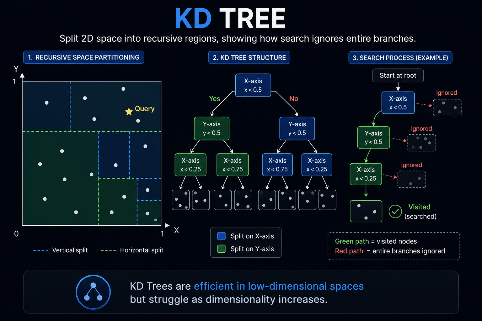
KD Trees: Organizing Space
If checking every vector is inefficient, perhaps we can organize vectors into a structure that allows large portions of the search space to be ignored.
That is exactly the idea behind KD Trees.
Rather than storing points in one enormous list, a KD Tree repeatedly divides space into smaller regions.
Imagine organizing houses by country, then city, then street.
If someone asks for an address in Paris, you don't inspect houses in Tokyo.
You immediately eliminate enormous portions of the search space.
KD Trees apply a similar strategy to vectors.
At low dimensions, this works remarkably well.
The problem is that modern embeddings don't live in two or three dimensions.
They often contain hundreds or even thousands of coordinates.
As dimensionality increases, the partitions become less effective. Eventually, the tree behaves almost like linear search again.
This phenomenon is known as the curse of dimensionality, and it fundamentally limits many classical search structures.
LSH: Finding Similarity Through Hashing
If partitioning space becomes difficult in high dimensions, perhaps we should stop trying to organize every point precisely.
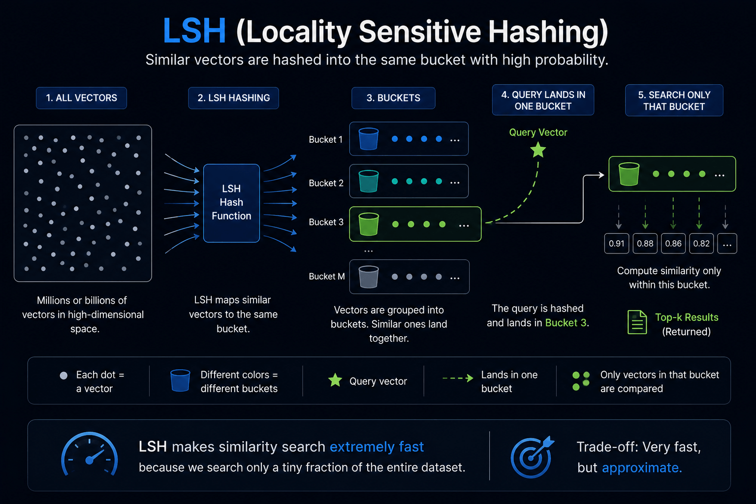
Locality Sensitive Hashing (LSH) takes a completely different approach.
Instead of searching every vector, it hashes similar vectors into the same buckets with high probability.
Think of it as assigning neighborhoods rather than exact addresses.
When a query arrives, the algorithm searches only within the most promising neighborhoods.
The search becomes dramatically faster because most of the database is ignored.
Of course, there's a tradeoff.
Occasionally, the true nearest neighbor may end up in a different bucket and never be examined.
That's why LSH is approximate.
But for many applications, the speed improvement is well worth the tiny loss in accuracy.
IVF: Searching Only the Right Neighborhood
One idea naturally follows from LSH.
Instead of randomly grouping vectors, what if we intentionally clustered them?
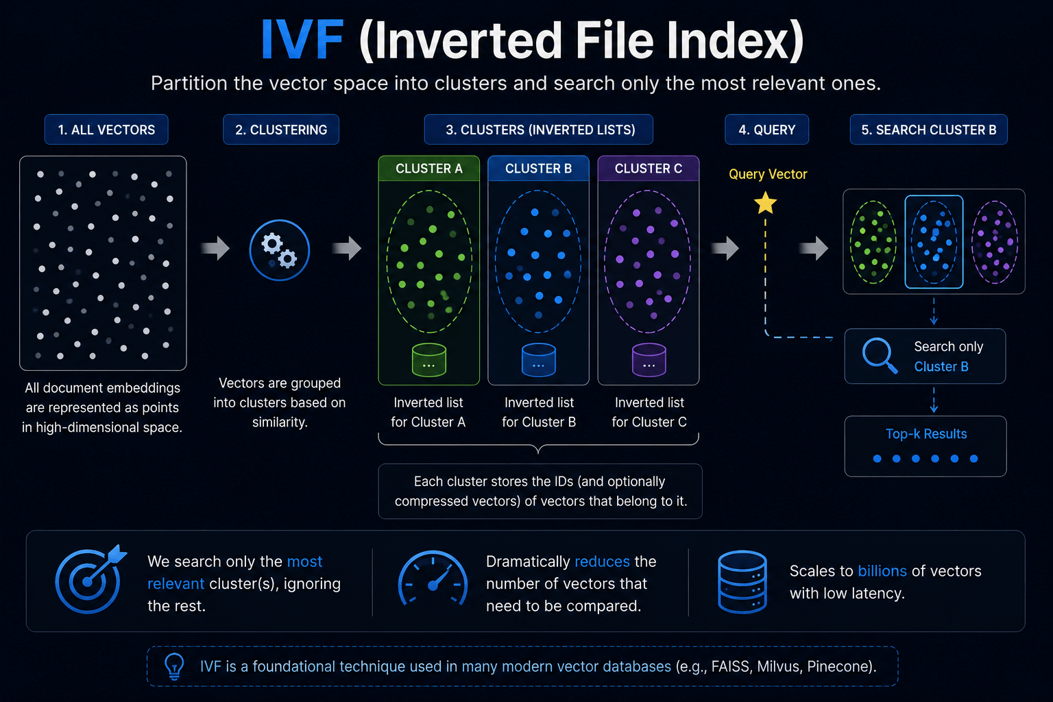
This is the foundation of the Inverted File Index (IVF).
During indexing, the database groups similar vectors together into clusters.
When a query arrives, it first identifies which clusters are closest to the query and searches only inside those clusters.
Most of the database is ignored entirely.
The larger the dataset becomes, the greater the benefit.
Instead of examining one billion vectors, the search may inspect only a few thousand candidates before computing exact similarity scores.
HNSW: Navigating a Graph Instead of Scanning Data
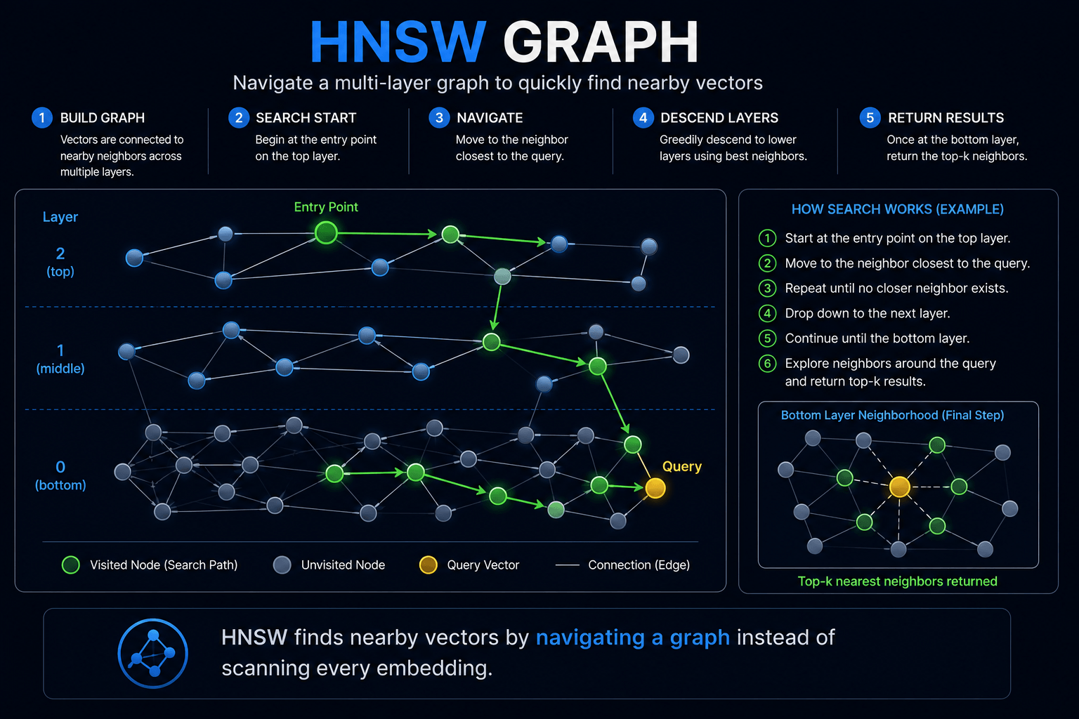
Today's production vector databases frequently rely on Hierarchical Navigable Small World (HNSW) graphs.
Rather than organizing vectors into trees or clusters, HNSW connects nearby vectors into a network.
Imagine standing in an unfamiliar city.
Instead of checking every street, you ask locals for directions.
Each person points you toward someone even closer to your destination.
Eventually, you arrive without ever exploring the entire city.
HNSW behaves similarly.
The algorithm starts from an entry point and repeatedly moves toward neighbors that appear increasingly similar to the query.
Because each step gets closer to the target, the search converges remarkably quickly.
This is one of the reasons HNSW has become the default index for many modern vector databases.
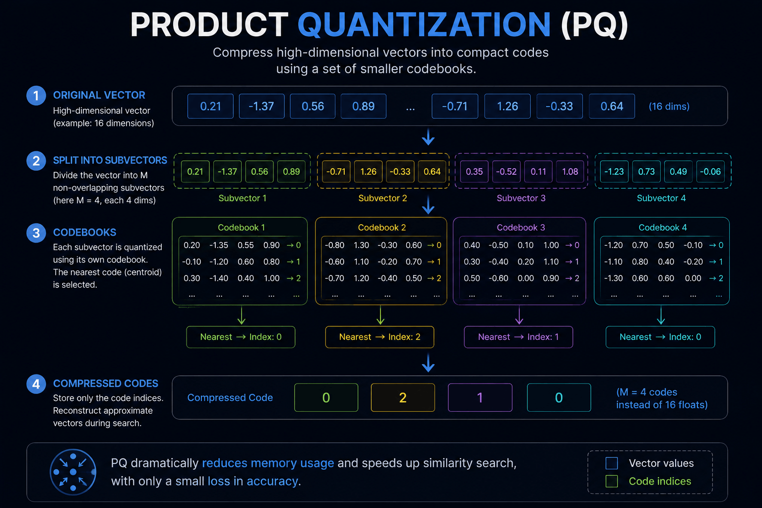
Product Quantization (PQ): Compressing Vectors
Searching billions of embeddings is only part of the challenge.
Storing them efficiently is equally important.
A single embedding may contain hundreds or thousands of floating-point numbers.
Multiply that by billions of documents and memory requirements become enormous.
Product Quantization (PQ) addresses this problem by compressing vectors into compact codes while preserving enough information for similarity search.
The compressed representation dramatically reduces memory usage and allows much larger datasets to fit into RAM or cache.
The database performs most searches on these compressed vectors before refining the final results using the original embeddings when necessary.
Compression introduces a small amount of approximation, but the infrastructure savings are substantial.
DiskANN: When RAM Is No Longer Enough
Even compressed vectors eventually outgrow available memory.
Large AI systems may store tens or hundreds of billions of embeddings.
Keeping everything in RAM becomes prohibitively expensive.
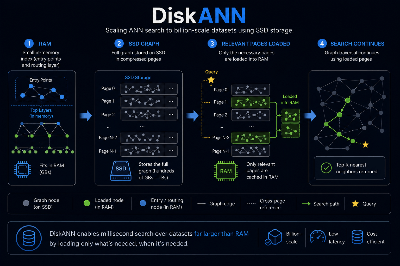
DiskANN extends approximate nearest neighbor search to SSD storage.
Rather than requiring the entire index to remain in memory, it intelligently loads only the portions needed during search.
The result is a system capable of searching datasets far larger than available RAM while maintaining remarkably low latency.
This approach has become increasingly important as enterprise knowledge bases, recommendation systems, and AI search engines continue growing.
Choosing the Right ANN Algorithm
Each algorithm exists because no single solution works best in every situation.
The remarkable thing about modern vector databases is that they rarely rely on just one of these ideas.
A production system might combine HNSW for navigation, PQ for compression, metadata filtering for narrowing the search space, and SSD-backed storage inspired by DiskANN to handle datasets that exceed available memory.
Each technique solves a different engineering problem, and together they make billion-scale semantic search practical.
Understanding these algorithms explains why vector search feels almost instantaneous—even when the database contains more information than a human could read in several lifetimes.
The next question is no longer how vector search works, but which implementation is right for your own applications. In the next chapter, we'll compare the most popular vector databases—from pgvector and FAISS to Pinecone, Milvus, Qdrant, Weaviate, Redis, and Chroma—to understand where each one excels and where its tradeoffs begin.
🛠️ Book Worth Reading

Mining of Massive Datasets
Interested in the algorithms behind web-scale search and machine learning? Mining of Massive Datasets covers similarity search, LSH, recommendation systems, graph mining, and distributed data processing.
Try Mining of Massive Datasets8. Choosing the Right Vector Database8 min read
Before we compare anything...
One of the most common questions developers ask after learning how vector databases work is surprisingly simple:
"Which vector database should I use?"
It sounds like there should be a single correct answer.
There isn't.
Choosing a vector database is a bit like choosing a programming language or a cloud provider. Every system is optimized for different trade-offs. Some prioritize developer experience. Others focus on billion-scale datasets. Some integrate seamlessly into existing PostgreSQL deployments, while others are purpose-built for semantic search from the ground up.
A database that performs exceptionally well for a personal RAG project may become prohibitively expensive at enterprise scale. Likewise, a system capable of indexing billions of vectors might be unnecessarily complex for a startup storing only a few thousand documents.
The goal, then, isn't to find the "best" vector database.
The goal is to find the one that best matches your workload.
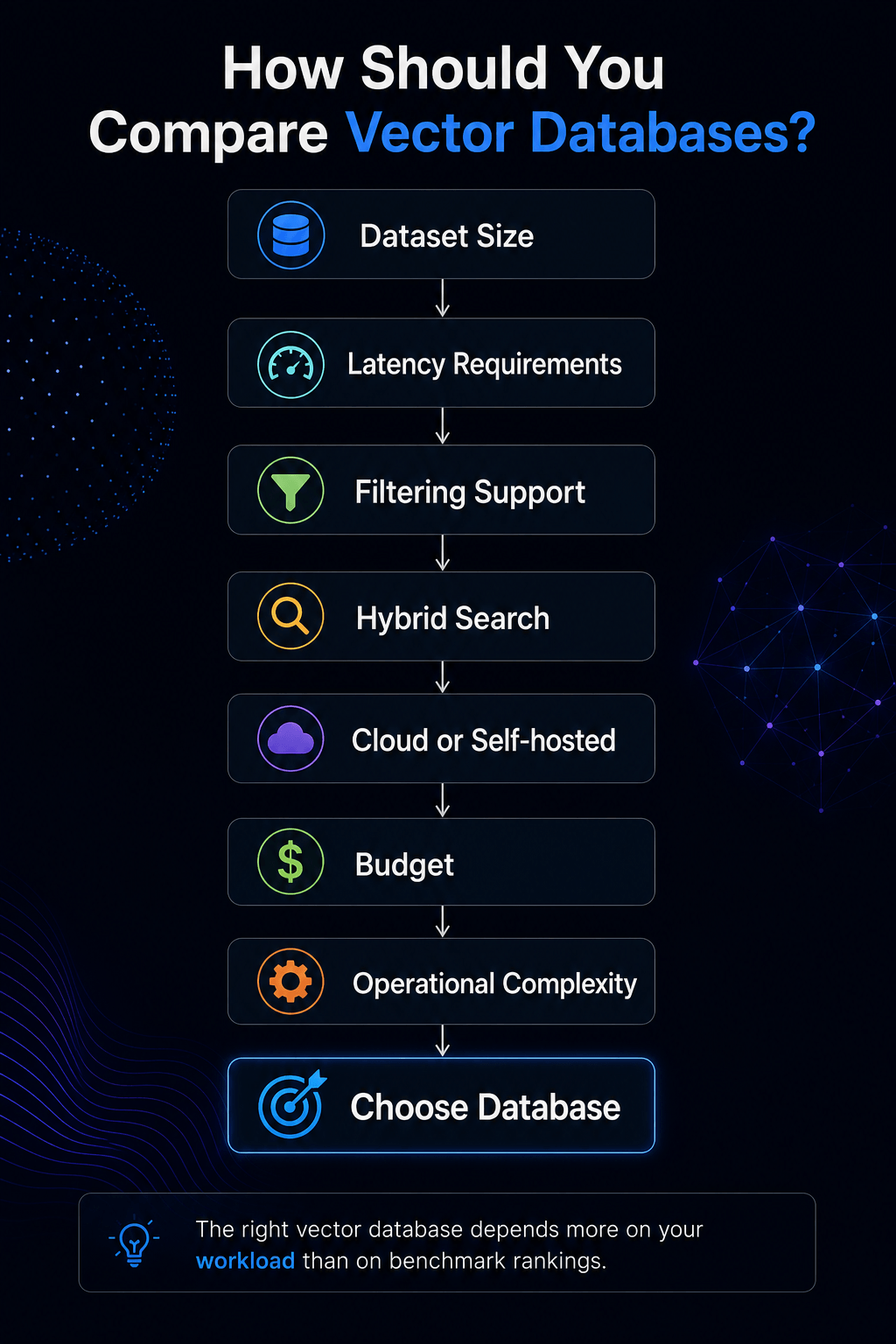
Before diving into individual products, it's helpful to understand the criteria that actually matter when evaluating a vector database.
What Actually Matters?
Benchmark charts often compare databases using queries per second or indexing speed. Those metrics are useful, but they rarely answer the questions most engineers care about.
Can the database handle metadata filtering efficiently?
Does it support hybrid search?
Can it scale across multiple machines?
Is it open source?
How difficult is it to operate in production?
How expensive does it become when your dataset grows from one million vectors to one billion?
These practical considerations often matter far more than small performance differences.
For the remainder of this section, we'll compare the most widely used vector databases using criteria that reflect real production deployments rather than isolated benchmark numbers.
Don't look for the database with the most ✓ marks.
Instead, find the one whose strengths align with your project.
A lightweight RAG prototype and a global recommendation system have very different requirements.
Pinecone
Pinecone is one of the most widely adopted managed vector databases and is often the first platform developers encounter when building Retrieval-Augmented Generation systems. Its biggest strength is simplicity. Developers can focus on building AI applications without worrying about index management, replication, scaling, or infrastructure.
The platform handles operational complexity automatically while providing excellent metadata filtering, hybrid search, and low-latency retrieval. This makes it particularly attractive for startups and enterprise teams that prefer managed services over operating distributed infrastructure.
The trade-off is cost. Managed convenience comes with recurring operational expenses, especially as datasets and query volumes increase.
For teams that prioritize developer productivity over infrastructure management, Pinecone remains one of the strongest choices available.
🛠️ Quick Verdict
Pinecone
✅ Best for production SaaS ✅ Excellent developer experience ✅ Fully managed ⚠️ Higher long-term cost Recommended if you're building production RAG systems and don't want to manage infrastructure.
Try PineconeQdrant
Qdrant has become one of the fastest-growing open-source vector databases, largely because it combines excellent performance with a developer-friendly architecture. Unlike many traditional databases that later added vector support, Qdrant was designed specifically for semantic search.
Its metadata filtering is among the strongest in the industry, making it particularly well suited for Retrieval-Augmented Generation, recommendation systems, and enterprise document search.
Developers can self-host Qdrant for complete control or use its managed cloud offering when operational simplicity becomes more important.
For many teams, Qdrant offers one of the best balances between performance, flexibility, and operational cost.
Quick Verdict
Best balance between open source and production readiness.
Milvus
Milvus is designed for scale.
When organizations need to index hundreds of millions—or even billions—of embeddings, Milvus becomes an attractive option because its architecture was built specifically for distributed deployments.
Its indexing capabilities, scalability, and support for multiple ANN algorithms make it particularly appealing for large AI platforms and research organizations.
The downside is operational complexity. Running Milvus effectively often requires more infrastructure expertise than lightweight alternatives.
For enterprise AI infrastructure, however, that investment can be worthwhile.
Weaviate
Weaviate takes a slightly different approach by offering a broader ecosystem around semantic search. Beyond vector storage, it includes modules for knowledge graphs, multimodal retrieval, and integrations with popular embedding providers.
Developers building sophisticated semantic applications often appreciate its rich API design and extensibility.
The learning curve is slightly steeper than lightweight databases, but the flexibility is substantial.
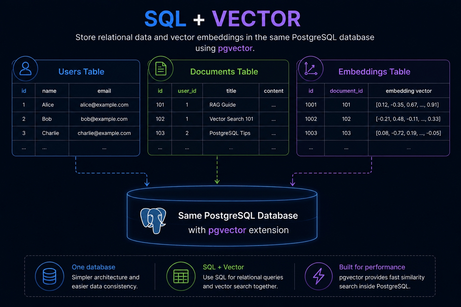
pgvector
Not every application needs a dedicated vector database.
If your project already relies heavily on PostgreSQL, adding pgvector can dramatically simplify your architecture.
Instead of operating two separate databases—one relational and one vector—you can store embeddings alongside traditional relational data.
For small to medium-sized applications, this can be an elegant solution.
Eventually, however, very large vector workloads begin to expose PostgreSQL's limitations compared to specialized vector search engines.
Redis
Redis is traditionally known as an in-memory key-value store, but recent versions have introduced vector search capabilities.
Its greatest strength remains latency.
Applications requiring extremely fast retrieval—particularly when vectors are already closely tied to cached application state—can benefit from Redis.
For large document retrieval systems, however, dedicated vector databases generally provide richer indexing and search capabilities.
FAISS
FAISS is not a database.
It's an indexing library.
This distinction is important.
FAISS gives developers direct access to state-of-the-art similarity search algorithms, making it extremely popular in research and custom infrastructure.
What it doesn't provide is everything surrounding those algorithms.
There is no built-in API, authentication, replication, distributed management, or metadata filtering.
If you're building your own search engine from scratch, FAISS is an outstanding foundation.
If you're deploying a production enterprise RAG system, you'll usually want additional infrastructure around it.
FAISS is the engine.
A vector database is the entire car.
Chroma
Chroma focuses on simplicity.
Getting started takes only a few minutes, making it ideal for tutorials, prototypes, notebooks, and local AI experiments.
Many developers begin their vector search journey with Chroma before eventually migrating to larger production systems.
Its limitations become apparent primarily when scaling beyond modest workloads.
Which One Should You Choose?
There is no universally best vector database.
Instead, the decision depends on the scale of your application, operational expertise, infrastructure preferences, and budget.
The recommendations below summarize common production scenarios.
Try this to find suitable Vector DB
The comparison we've made so far assumes that your vector database is already working correctly.
In practice, however, many production systems fail not because the database is slow, but because they're configured poorly.
Choosing the right chunk size, selecting an appropriate embedding model, designing metadata correctly, monitoring recall, controlling latency, and balancing cost all have a far greater impact on retrieval quality than simply picking one vector database over another.
In the next chapter, we'll explore the production mistakes that quietly break otherwise well-designed RAG systems—and how experienced engineering teams avoid them.
9. 10 Mistakes That Quietly Destroy RAG Performance9 min read
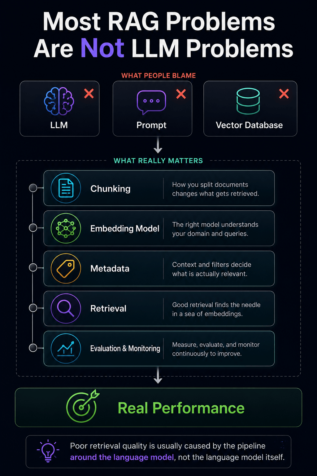
Most teams blame the LLM. The real problem is usually somewhere else.
By now, we've explored the entire retrieval pipeline. We know how embeddings are created, how vector databases organize them, how Approximate Nearest Neighbor algorithms retrieve similar documents, and how modern RAG systems assemble context before sending it to a language model.
At this point, it might seem that building a Retrieval-Augmented Generation system is simply a matter of connecting these components together.
In reality, that's where the difficult part begins.
Many production teams spend weeks optimizing prompts, experimenting with larger language models, or switching vector databases in search of better answers. Yet the underlying problem often has nothing to do with the model itself.
Poor chunking can hide the information the model needs.
An unsuitable embedding model can separate related concepts.
Missing metadata can cause irrelevant documents to appear in search results.
A retrieval pipeline without reranking may retrieve technically similar documents that fail to answer the user's question.
These issues rarely produce obvious failures. Instead, they quietly reduce answer quality, increase hallucinations, and slowly erode user trust.
This section covers ten of the most common mistakes engineers make when deploying vector search systems—and how to avoid them before they reach production.
Mistake 1 — Choosing the Wrong Chunk Size
One of the first design decisions in any Retrieval-Augmented Generation system is how documents should be divided before embeddings are created.
Many teams underestimate how important this step is.
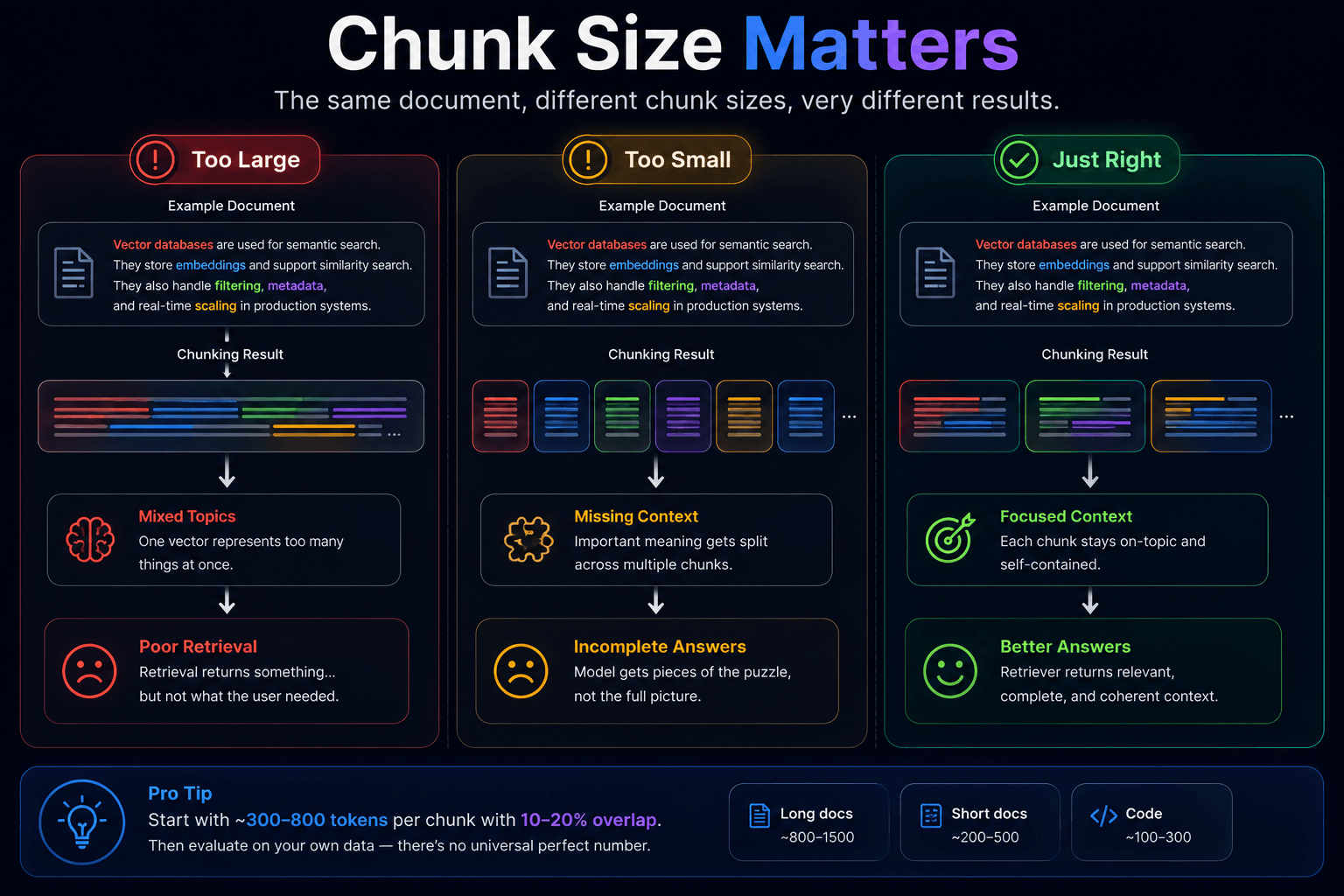
If chunks are too large, each embedding represents several unrelated topics at once. A single vector may contain information about installation, configuration, troubleshooting, and licensing, making it difficult for semantic search to retrieve precisely the section a user needs.
If chunks are too small, the opposite problem appears. Important context becomes fragmented across multiple vectors. The retriever may return one paragraph while missing the explanation immediately before or after it.
There is no universally correct chunk size. The optimal value depends on the structure of your documents, the embedding model, and the type of questions users ask.
The important lesson is that chunking should be treated as an engineering decision rather than an arbitrary preprocessing step.
Document Chunk Simulator
⚠️ Too Small
- Context loss
- More embeddings
- More API cost
Mistake 2 — Using the Wrong Embedding Model
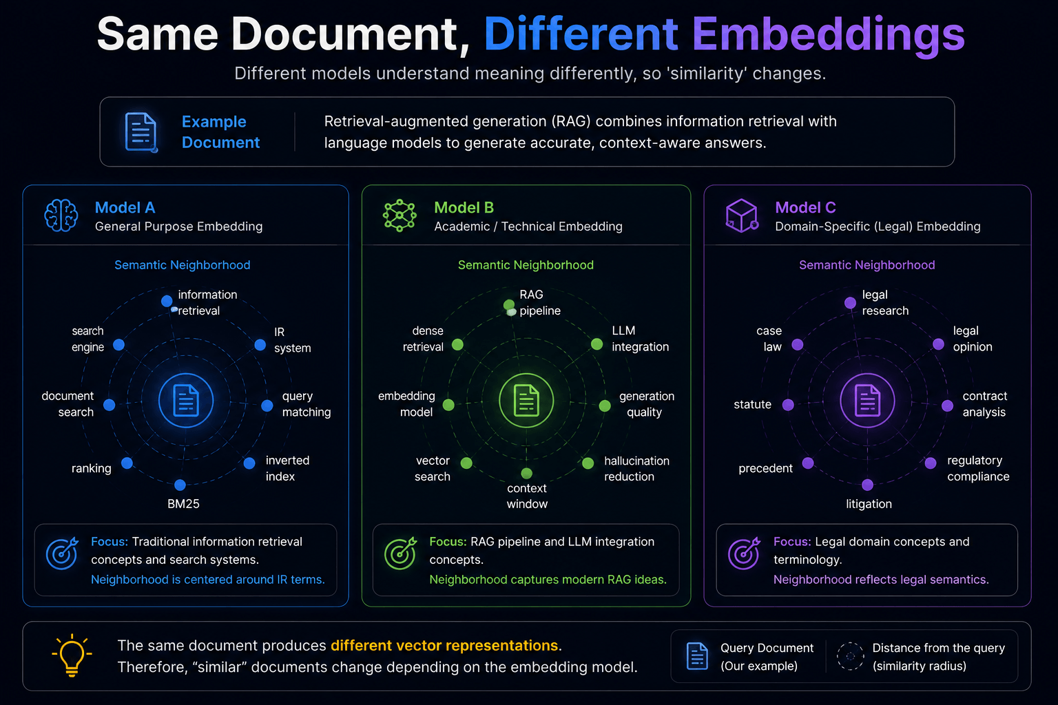
Not all embedding models understand language in the same way.
Some are optimized for short search queries.
Others perform better on scientific literature.
Some excel at multilingual retrieval, while others are trained primarily on English text.
Selecting an embedding model simply because it appears at the top of a benchmark leaderboard can produce disappointing results if the benchmark doesn't resemble your own workload.
Always evaluate embedding models using representative documents from your application rather than relying solely on public rankings.
Mistake 3 — Ignoring Metadata
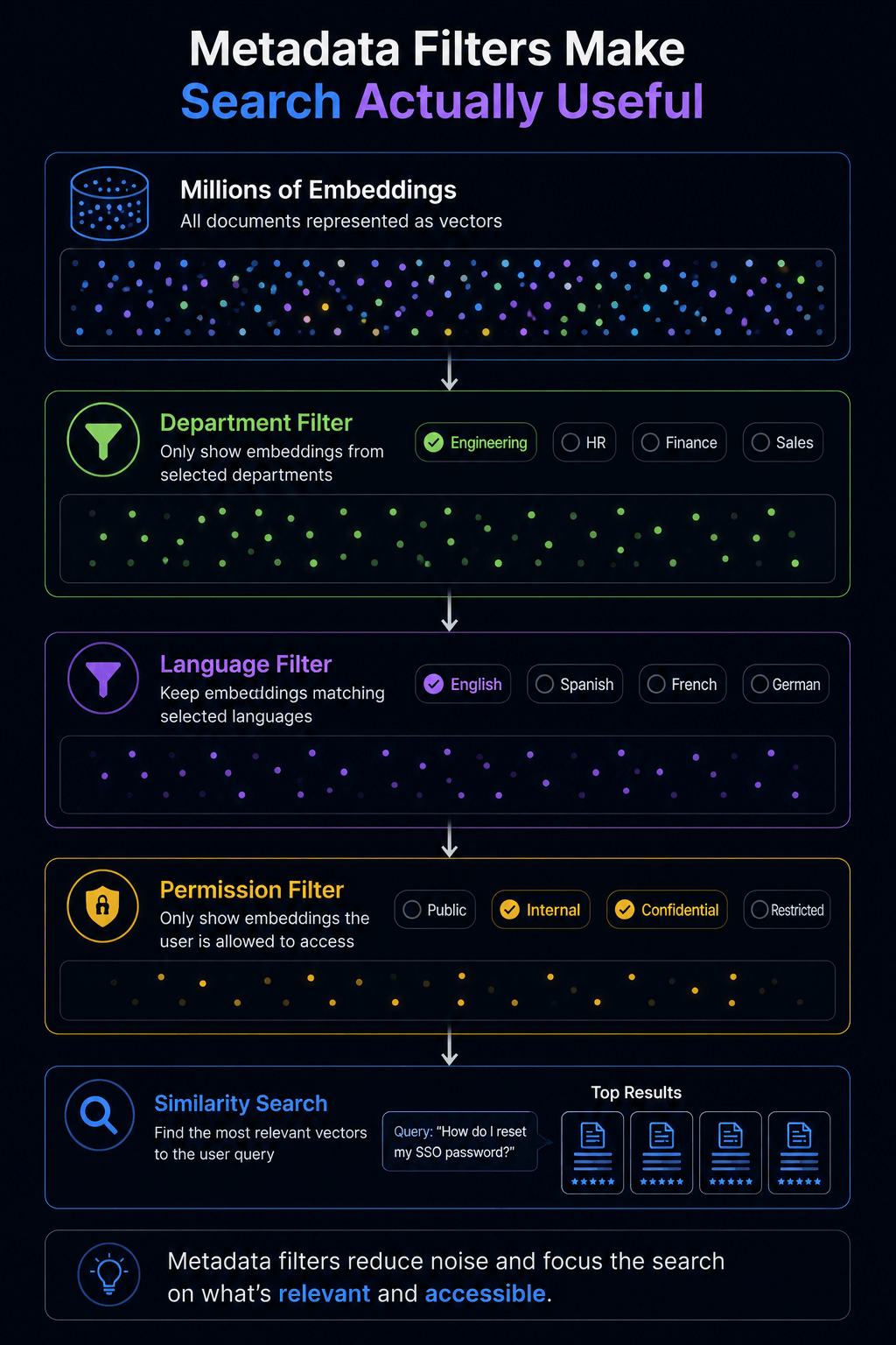
Semantic similarity is only one signal.
Context is equally important.
Suppose an employee searches for internal HR policies.
Without metadata filtering, the retriever may return engineering documentation that happens to discuss similar concepts.
Metadata such as department, language, publication date, customer account, access permissions, or document type often determines whether retrieved information is actually useful.
Strong production systems combine semantic search with structured filtering.
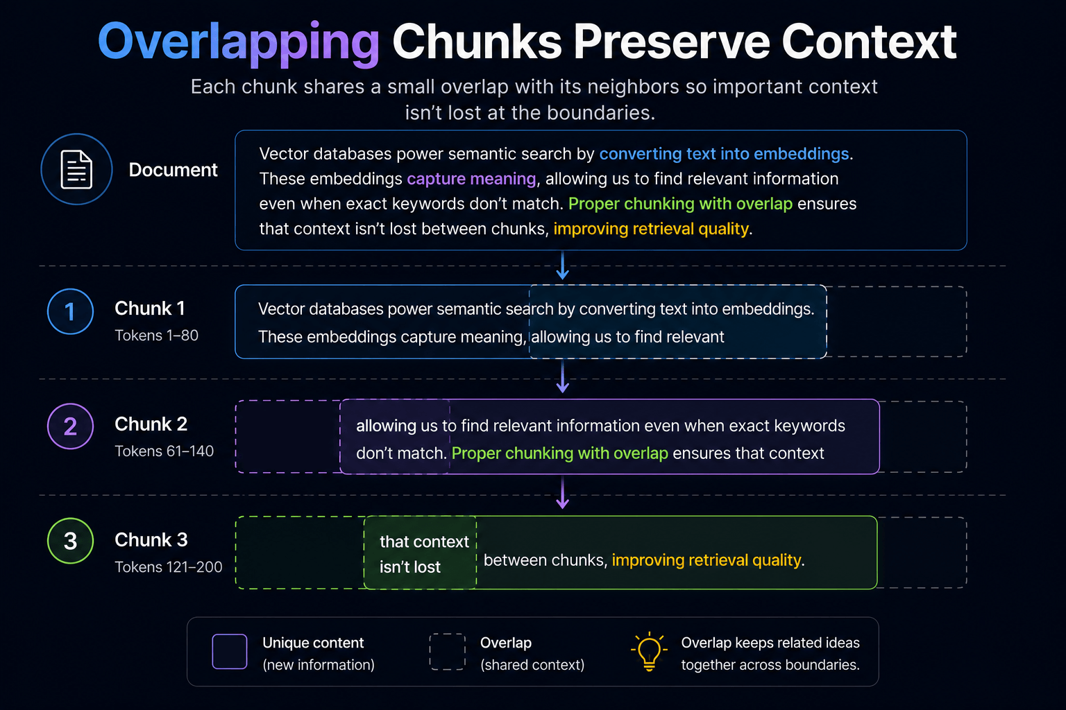
Mistake 4 — Forgetting Overlap Between Chunks
Documents rarely divide neatly into independent sections.
Important ideas often span multiple paragraphs.
Splitting documents without overlap can accidentally separate definitions from explanations, questions from answers, or code from accompanying documentation.
A small overlap between consecutive chunks helps preserve continuity while maintaining retrieval precision.
The exact amount depends on the application, but ignoring overlap entirely often produces incomplete answers.
Mistake 5 — Skipping Reranking
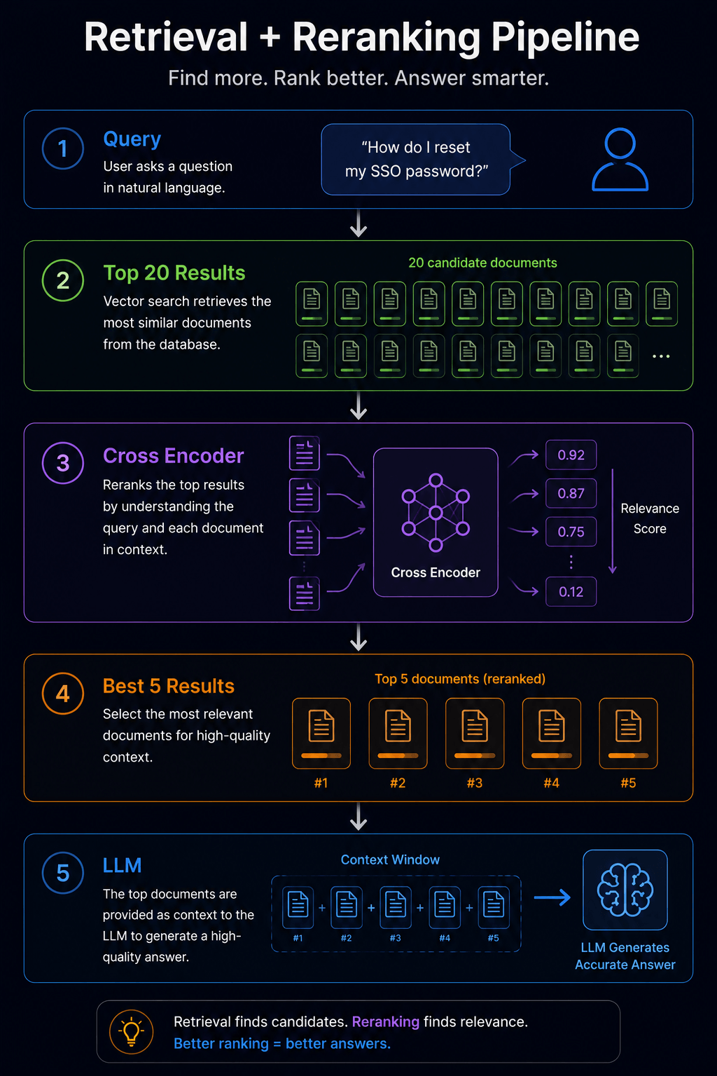
Initial retrieval identifies candidate documents.
That doesn't necessarily mean the best document appears first.
Modern production systems frequently retrieve twenty or thirty candidates before using a reranking model to reorder them according to the user's actual intent.
Reranking introduces a second stage of reasoning that often improves answer quality dramatically, particularly for complex enterprise knowledge bases.
Many teams never implement this second stage and unknowingly leave significant retrieval performance on the table.
Mistake 6 — Choosing the Wrong Similarity Metric
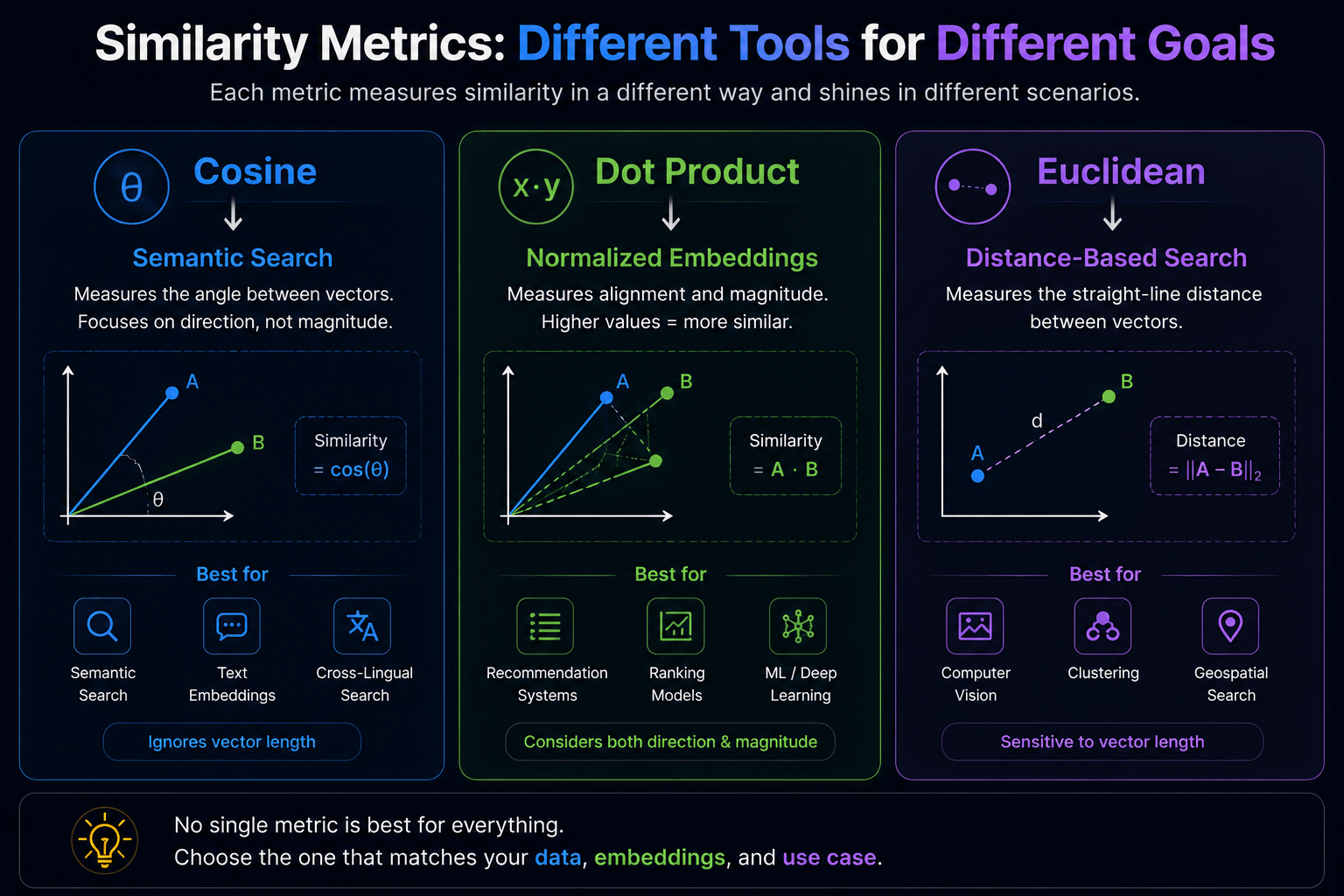
Earlier in this article we explored cosine similarity, Euclidean distance, and dot product.
Selecting the wrong metric for a particular embedding model can reduce retrieval quality even when everything else is configured correctly.
Fortunately, most modern embedding providers document which similarity metric should be used.
Rather than experimenting randomly, begin with the recommendation supplied by the embedding model itself.
Mistake 7 — Forgetting Caching
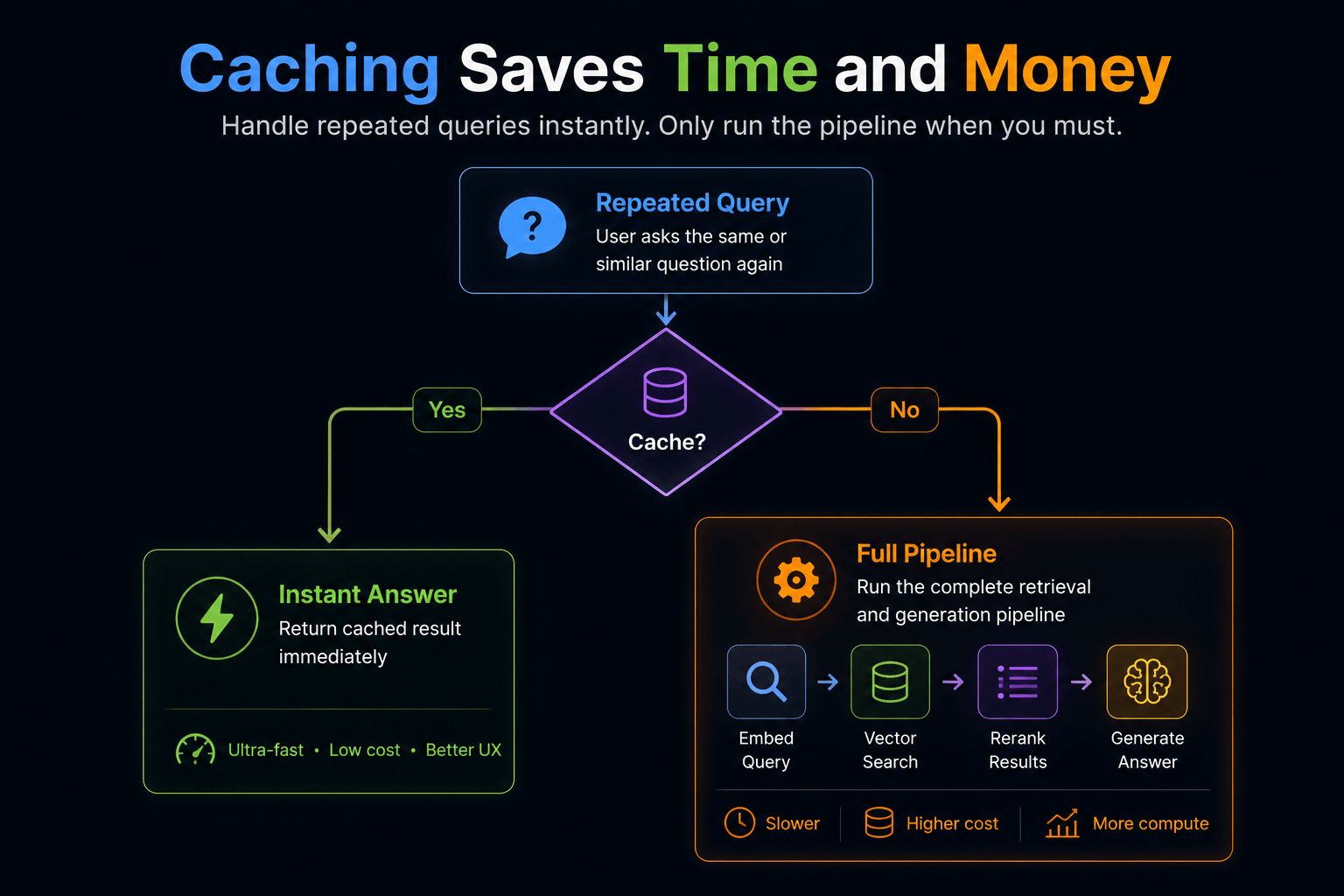
Many user questions repeat.
Customer support systems receive identical requests every day.
Internal knowledge assistants answer the same engineering questions repeatedly.
Without caching, every repeated query triggers another embedding request, another vector search, and another language model completion.
Caching popular queries dramatically reduces latency while lowering infrastructure costs.
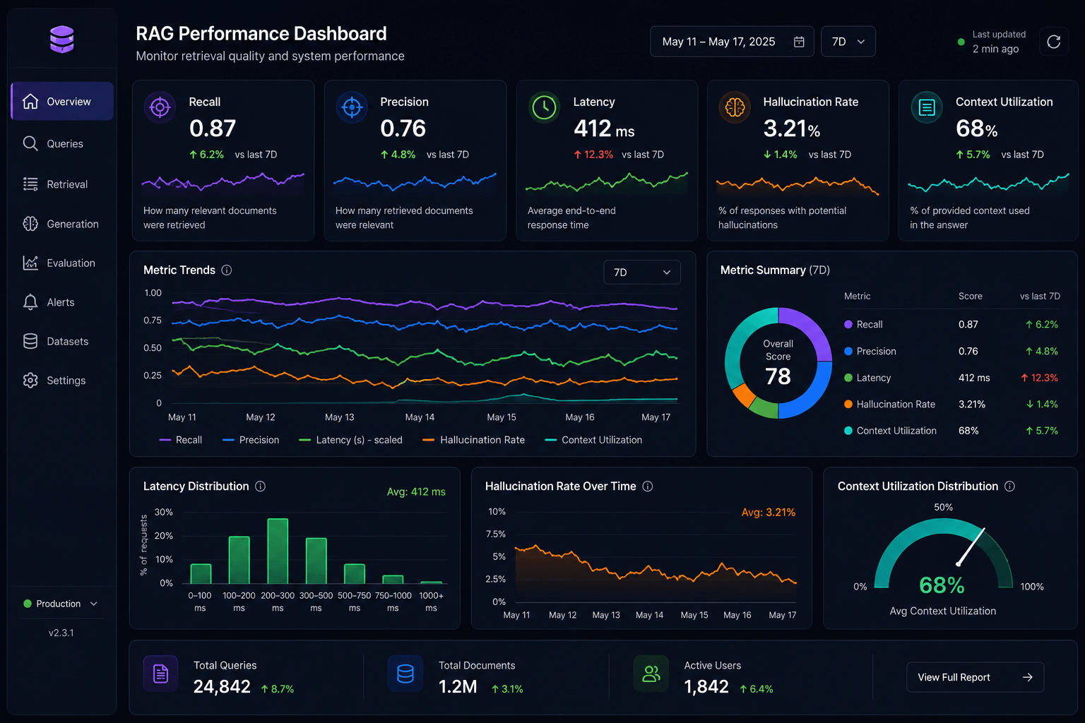
Mistake 8 — Never Monitoring Retrieval Quality
Many teams monitor CPU usage, latency, and API costs.
Far fewer monitor retrieval quality itself.
A production RAG system should continuously measure metrics such as recall, precision, latency, retrieval success rate, and answer quality.
Otherwise, performance can quietly deteriorate as documents change, embedding models evolve, or user behavior shifts.
Mistake 9 — Never Versioning Embeddings
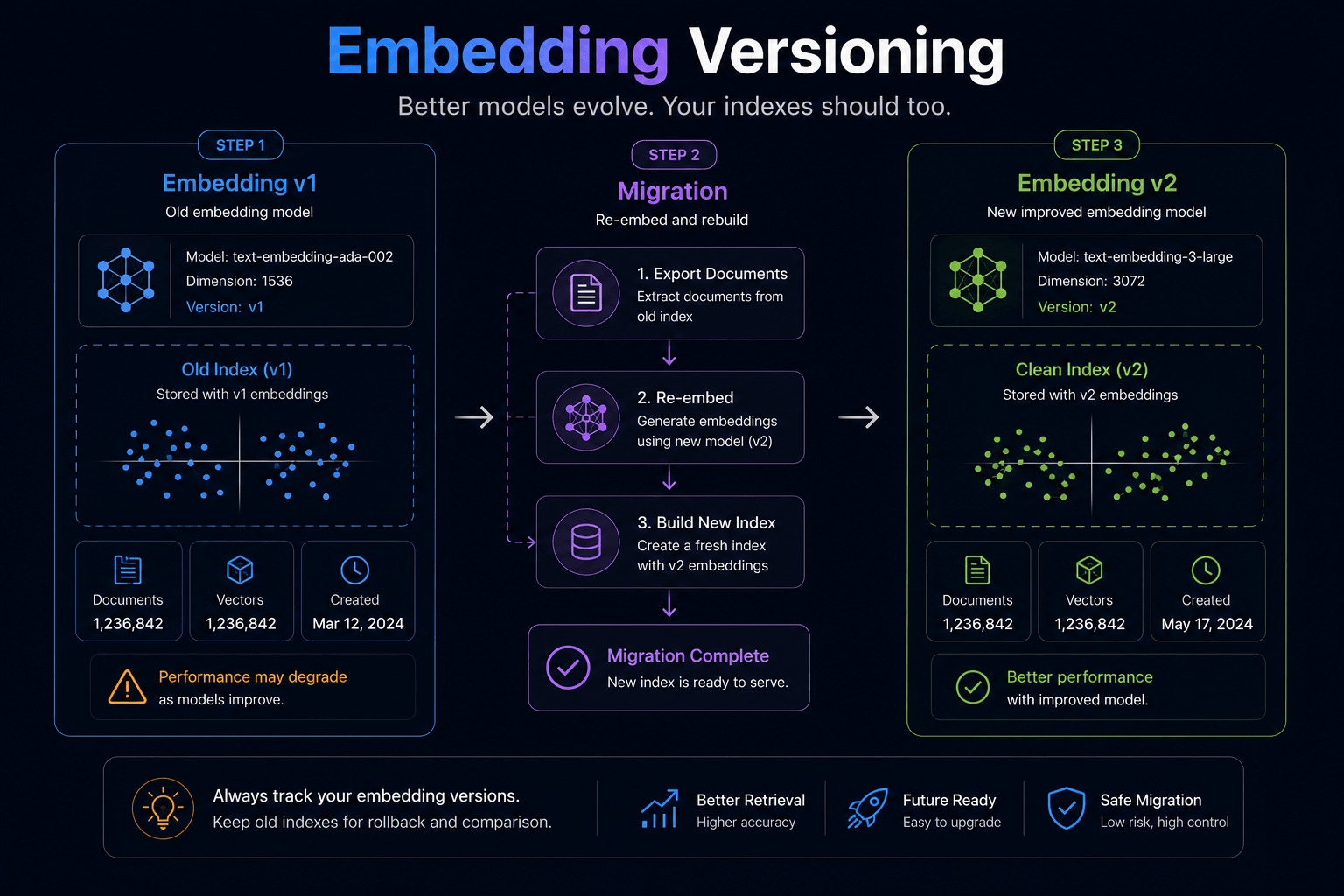
Embedding models improve continuously.
Eventually, you'll want to upgrade.
Without versioning, old and new embeddings become mixed together inside the same database.
The result is inconsistent retrieval behavior that's difficult to debug.
Production systems should treat embeddings as versioned artifacts, just like machine learning models or database schemas.
Mistake 10 — Never Building an Evaluation Dataset
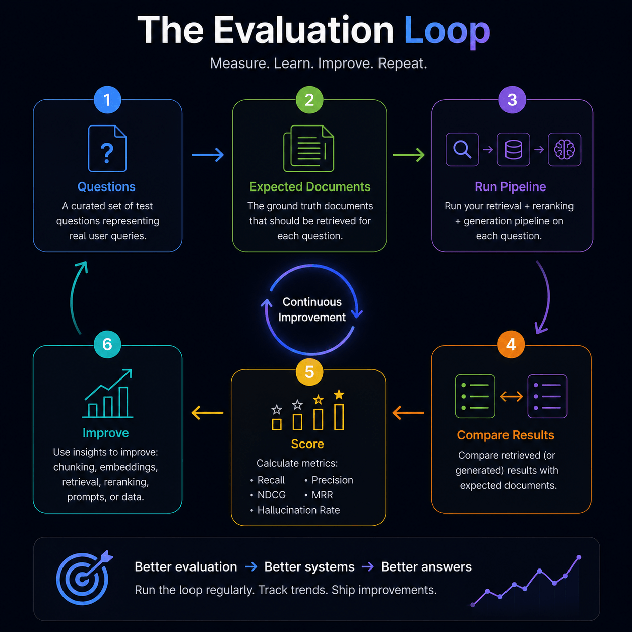
Perhaps the biggest mistake of all is assuming retrieval quality based on intuition.
Without an evaluation dataset, every improvement becomes subjective.
Did the new embedding model help?
Did chunk overlap improve retrieval?
Did reranking actually increase answer quality?
Nobody knows.
Successful AI teams maintain a collection of representative questions with expected answers.
Every pipeline change is evaluated against this benchmark before deployment.
Only then can retrieval quality improve systematically rather than accidentally.
Before shipping your RAG system, ask yourself:
The remarkable thing about vector search is that it continues to evolve rapidly. New indexing algorithms, multimodal embeddings, agent memory systems, hybrid retrieval techniques, and learned indexes are reshaping what semantic search can accomplish.
So where is all of this heading?
The next chapter explores the future of vector search—and why vector databases may become the long-term memory layer for the next generation of AI systems.
10. Beyond Vector Databases: The Future of AI Memory9 min read
For most of computing history, databases have existed for one purpose: storing information so that humans or software can retrieve it later. Whether the underlying technology was relational databases, document stores, graph databases, or vector indexes, the objective remained largely the same—persist data and return it when asked.
Modern AI is beginning to change that assumption.
Large language models are no longer passive systems waiting for queries. They plan tasks, use external tools, write code, collaborate with other agents, and maintain conversations that span days or even months. As these systems become more autonomous, memory stops being a convenience and becomes a fundamental capability.
The vector databases we use today are an important milestone, but they are unlikely to represent the final architecture of AI memory.
They're the beginning.
The next generation of intelligent systems will almost certainly require richer, more adaptive forms of knowledge representation than simple nearest-neighbor search alone.
This chapter explores where that evolution appears to be heading—not as science fiction, but as an engineering roadmap already taking shape across research labs and production AI systems.
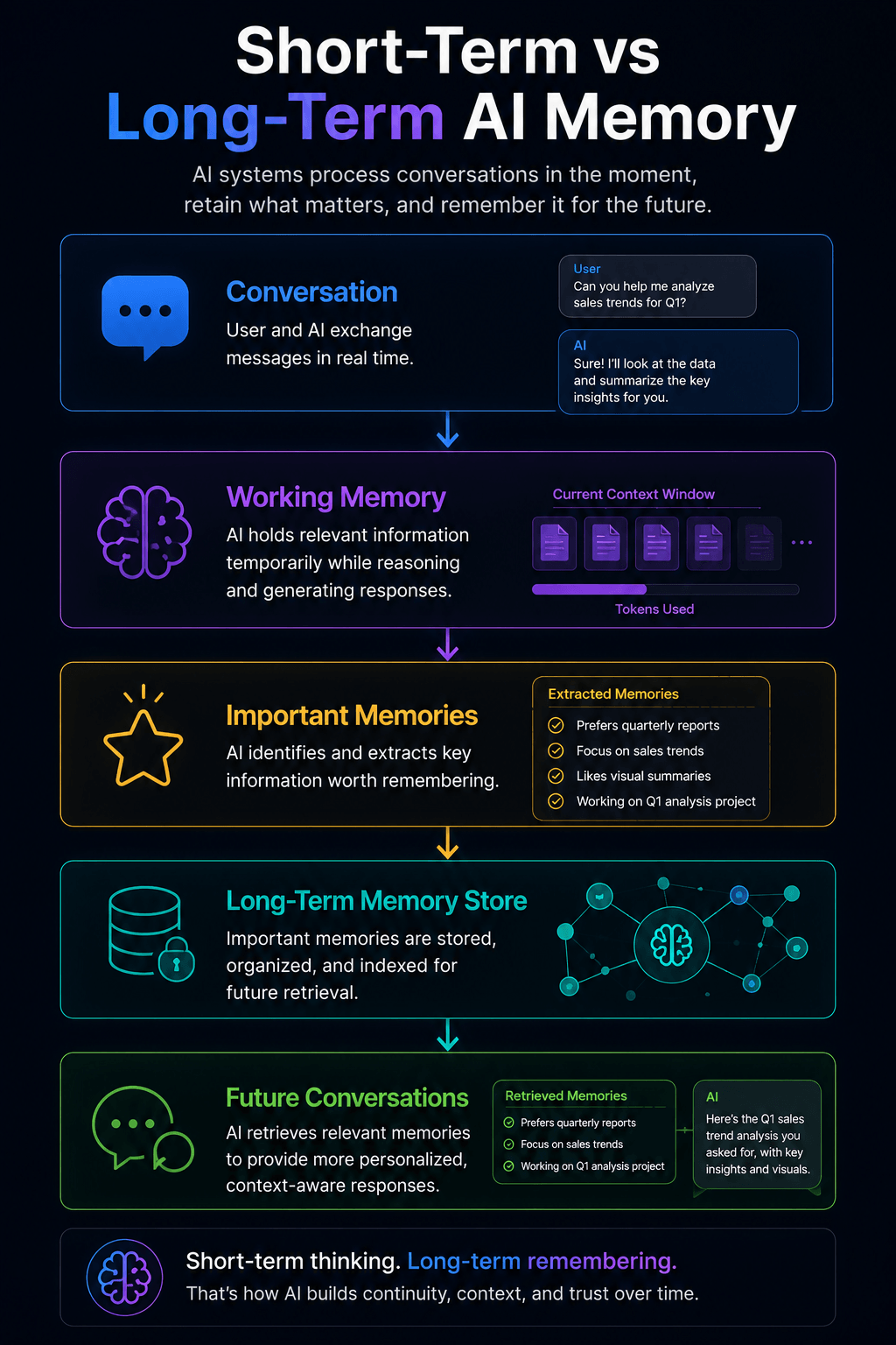
Prediction One — AI Will Remember Conversations Across Months
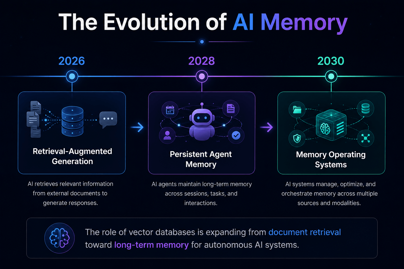
Today's Retrieval-Augmented Generation systems retrieve information from external documents.
Tomorrow's systems will retrieve information about you.
Imagine asking an AI assistant to continue a research project six months after your last conversation. Instead of starting from scratch, it remembers previous decisions, abandoned ideas, preferred writing styles, code architectures, and unresolved questions.
This isn't simply conversation history.
It is persistent memory.
Rather than treating every interaction as independent, future AI systems will maintain evolving knowledge about ongoing projects, organizations, and individuals.
Vector databases are already providing the foundation for many of these memory systems, but future architectures will likely organize memories according to importance, recency, confidence, and long-term relevance rather than storing every interaction equally.
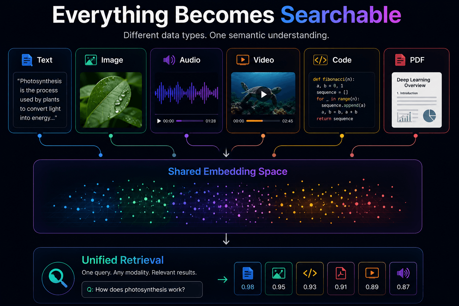
Prediction Two — Retrieval Will Become Fully Multimodal
Most retrieval systems today search text.
The next generation will search everything.
A design document will retrieve relevant diagrams.
An image will locate matching videos.
A voice recording will retrieve source code.
A photograph of a machine part may instantly locate engineering manuals, maintenance logs, CAD drawings, warranty documents, and previous repair reports.
The underlying principle remains the same: represent different types of information within a shared semantic space where meaning—not file format—determines proximity.
As multimodal embedding models improve, vector databases will evolve into unified search systems capable of retrieving text, images, audio, video, source code, 3D models, and sensor data using the same retrieval pipeline.
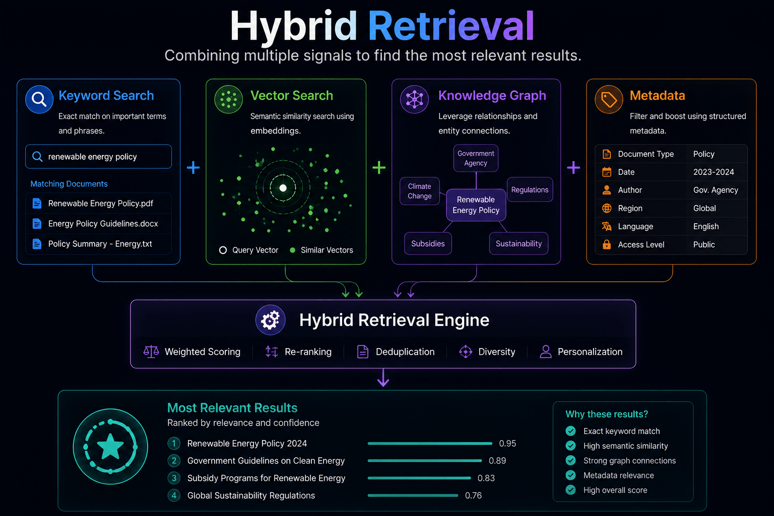
Prediction Three — Hybrid Search Will Become the Default
The debate between keyword search and semantic search is already beginning to fade.
Production systems increasingly combine both.
Keyword search excels when precision matters.
Semantic search excels when intent matters.
Metadata filtering provides contextual constraints.
Knowledge graphs contribute explicit relationships.
Future retrieval systems will combine all of these signals automatically.
Rather than choosing one retrieval method, the system will determine which combination produces the highest confidence answer.
From the user's perspective, there will simply be "search."
The underlying complexity will disappear.
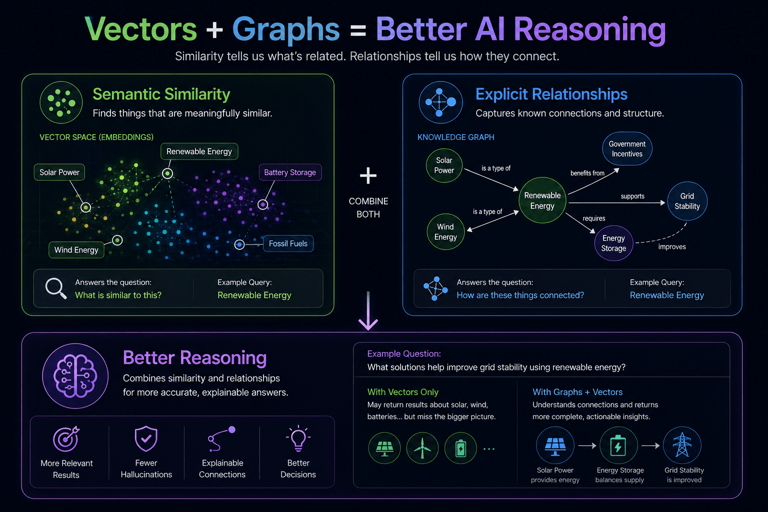
Prediction Four — Knowledge Graphs Will Return
For several years, vector databases dominated discussions around AI retrieval.
At the same time, knowledge graphs continued solving a different class of problems.
Graphs explicitly represent relationships.
Vectors capture similarity.
These are not competing ideas.
They are complementary.
Similarity tells us what feels related.
Graphs explain how things are related.
Future AI systems will increasingly combine both representations.
The vector database identifies candidate knowledge.
The graph validates relationships.
The language model reasons over both.
Instead of replacing one another, these technologies are converging into richer knowledge architectures.
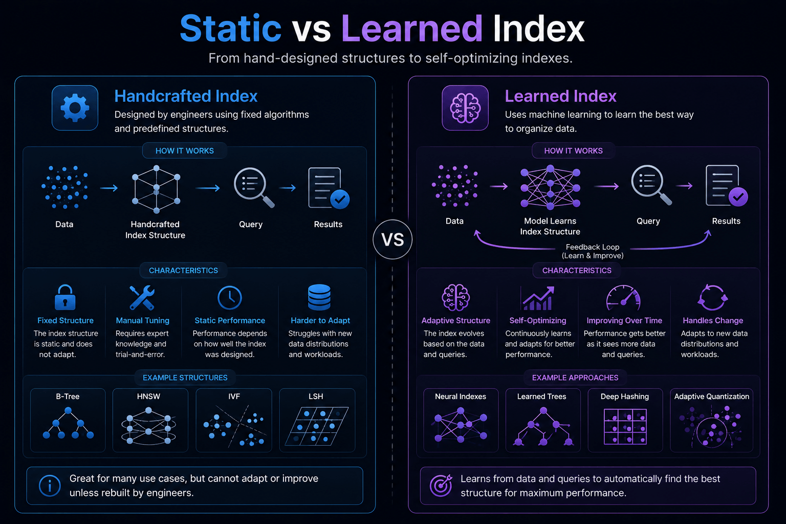
Prediction Five — Learned Indexes Will Replace Hand-Designed Structures
Today's vector databases rely on carefully engineered indexing algorithms such as HNSW, IVF, Product Quantization, and DiskANN.
These algorithms are remarkable achievements.
Yet they remain handcrafted solutions designed by engineers.
A growing body of research explores a different possibility: indexes that learn how to organize data automatically.
Rather than manually selecting graph structures or clustering strategies, future databases may train neural models that continuously optimize retrieval performance based on real workloads.
Instead of adapting applications to indexes, indexes will adapt themselves to applications.
Prediction Six — AI Will Need Memory Operating Systems
Today's operating systems manage CPU scheduling, memory allocation, storage, networking, and security.
Future AI systems may require something entirely different.
Memory management.
Imagine an autonomous research agent operating continuously for several years.
It cannot remember everything forever.
Some memories become obsolete.
Some become more important.
Some require compression.
Others must be forgotten.
Managing this lifecycle resembles operating system design far more than database engineering.
Future AI infrastructure may include dedicated memory managers responsible for deciding what should be remembered, compressed, archived, summarized, or discarded.
Vector databases could become only one component within a much larger memory architecture.
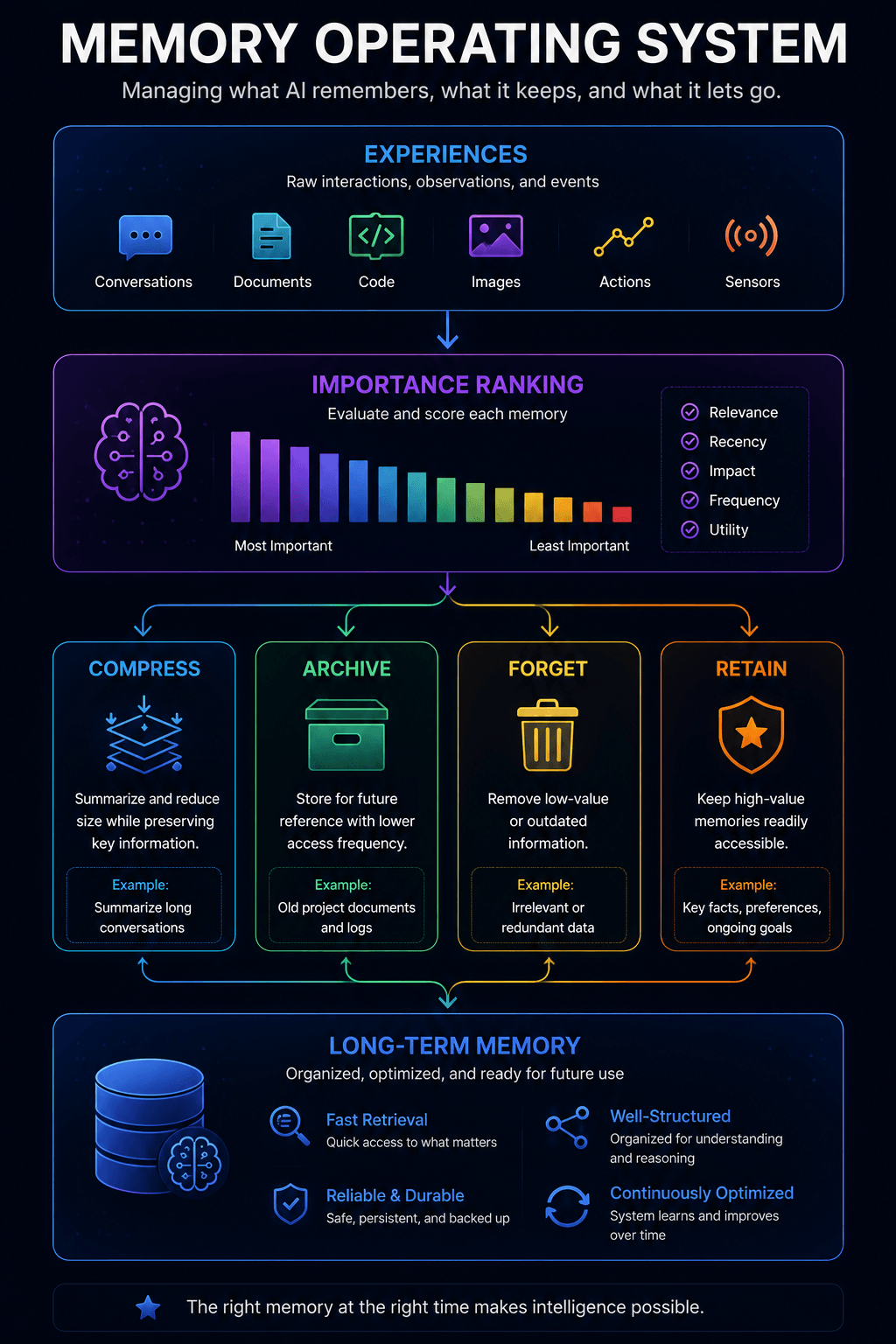
Prediction Seven — Retrieval Will Become Invisible
The most successful infrastructure eventually disappears.
Nobody thinks about DNS before opening a website.
Few developers think about CPU cache hierarchies while writing software.
Vector retrieval is likely heading toward the same fate.
Application developers won't ask whether a query used HNSW, DiskANN, lexical search, graph traversal, reranking, or metadata filtering.
They'll simply ask a question.
The infrastructure beneath the surface will determine the optimal retrieval strategy automatically.
Semantic retrieval will become an invisible layer of modern computing.
THE BIG IDEA
Users don't care how information is retrieved.
They care whether the answer is correct.
So… Are Vector Databases the Future?
Ironically, after spending thousands of words discussing vector databases, the answer is both yes and no.
Yes, because they introduced a fundamentally new way of representing and retrieving information based on meaning rather than exact words.
No, because they are unlikely to remain isolated systems.
Instead, they are gradually becoming one component inside a broader AI memory architecture that combines semantic search, structured metadata, knowledge graphs, multimodal retrieval, learned indexes, reasoning systems, and persistent long-term memory.
The future isn't a world where vector databases replace SQL.
It's a world where AI systems use multiple specialized memory layers, each solving a different part of the retrieval problem.
Vector databases won't replace existing databases.
They will become the semantic memory layer that allows intelligent systems to understand, retrieve, and reason over information in ways traditional databases never could.
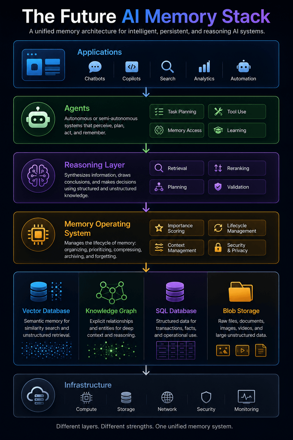
We've now followed the entire journey—from the limitations of keyword search to embeddings, similarity search, vector databases, Retrieval-Augmented Generation, production engineering, optimization, and finally the future of AI memory.
Before we finish, let's compress everything you've learned into a single visual page that connects every concept in this article into one mental model. That one-page recap is designed to be bookmarked, shared, and revisited whenever you need to understand how modern semantic search systems fit together.
11. Everything We Learned — One Page3 min read
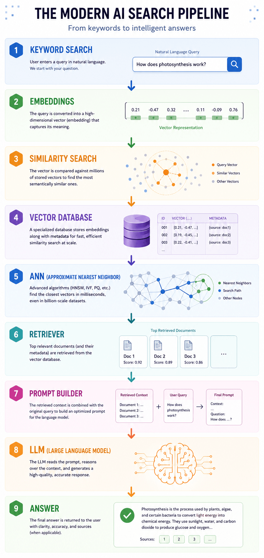
Quick Definitions
Which Vector Database Should I Use?
ANN Algorithms at a Glance
Complete RAG Pipeline
Steps in RAG
Documents
Chunking
Embeddings
Vector Database
Retriever
Prompt Builder
LLM
Answer
Key Takeaways
- Meaning can be represented mathematically.
- Embeddings allow semantic search instead of keyword matching.
- Vector databases make similarity search practical at scale.
- ANN algorithms enable millisecond retrieval across billions of vectors.
- RAG grounds language models in external knowledge.
- Retrieval quality often matters more than prompt engineering.
- Future AI systems will rely on persistent, multimodal memory.
:: Quick Knowledge Recap
What is a vector database?
A vector database is a specialized database designed to store, index, and search high-dimensional numerical representations called embeddings. Unlike traditional databases that retrieve records using exact matches or predefined conditions, vector databases retrieve information based on semantic similarity. This allows applications to find documents, images, code, or other content that expresses the same meaning as a user's query, even when the exact words differ. Modern AI systems use vector databases as the retrieval layer for semantic search, recommendation systems, Retrieval-Augmented Generation (RAG), and long-term AI memory.
Why do we need a vector database?
Traditional databases excel at storing structured information but struggle to understand meaning in natural language. A vector database solves this problem by storing embeddings instead of relying solely on keywords. It enables applications to search by intent rather than exact wording, making it essential for AI assistants, recommendation engines, semantic document search, and modern RAG systems.
What is an embedding?
An embedding is a numerical representation of a word, sentence, image, document, or other piece of information inside a high-dimensional mathematical space. You can think of it as the coordinates of meaning. Similar concepts are placed close together, while unrelated concepts are positioned farther apart. These coordinates make semantic search possible.
Are embeddings the same as vectors?
In practice, the terms are often used interchangeably. Technically, a vector is simply an ordered list of numbers, while an embedding is a vector that represents semantic meaning learned by a machine learning model. Every embedding is a vector, but not every vector is an embedding.
What is semantic search?
Semantic search retrieves results based on meaning rather than exact keyword matches. Instead of searching for identical words, it compares embeddings to determine which documents express concepts most similar to the user's query.
How does semantic search differ from keyword search?
Keyword search looks for matching words or phrases. Semantic search compares meanings using embeddings. Keyword search may miss documents that use different terminology, while semantic search can retrieve documents that discuss the same concept using different words.
What is cosine similarity?
Cosine similarity measures how closely two vectors point in the same direction. It ignores vector length and focuses entirely on orientation, making it one of the most common similarity metrics for normalized embeddings used in semantic search.
What is Euclidean distance?
Euclidean distance measures the straight-line distance between two vectors. It works well when absolute distance is meaningful, but for many embedding models, cosine similarity usually provides better semantic comparisons.
What is the dot product?
The dot product measures both direction and magnitude. Depending on the embedding model, it may be used as the preferred similarity metric because it incorporates vector length as well as alignment.
Which similarity metric is best?
There is no universally best metric. Most modern embedding models specify the recommended similarity function. Cosine similarity is widely used for normalized embeddings, while dot product is common for several transformer-based models. Euclidean distance is less common for modern semantic retrieval.
What is Approximate Nearest Neighbor (ANN) search?
ANN search finds vectors that are approximately the closest instead of computing the exact nearest neighbors. This dramatically reduces search time while sacrificing only a tiny amount of accuracy, making billion-scale semantic search practical.
Why not compare every vector directly?
Linear search requires comparing the query against every stored embedding. While this guarantees perfect accuracy, it becomes computationally expensive for datasets containing millions or billions of vectors. ANN algorithms solve this scalability problem.
What is HNSW?
Hierarchical Navigable Small World (HNSW) is a graph-based ANN algorithm that connects similar vectors together. Instead of scanning the entire dataset, search navigates this graph to quickly find nearby vectors, offering excellent speed and recall.
What is IVF?
Inverted File Index (IVF) clusters embeddings into groups. During search, only the most relevant clusters are examined rather than the entire dataset, greatly improving retrieval speed.
What is Product Quantization (PQ)?
Product Quantization compresses embeddings into compact representations. This reduces memory usage significantly while preserving most retrieval quality, making it possible to search extremely large datasets efficiently.
What is DiskANN?
DiskANN is an ANN algorithm designed for datasets too large to fit entirely into RAM. It stores graph structures on SSDs while intelligently loading only the portions required for each query.
What is Retrieval-Augmented Generation (RAG)?
Retrieval-Augmented Generation combines vector search with large language models. Before generating an answer, the system retrieves relevant documents from a vector database and includes them in the prompt, allowing the model to answer using external knowledge.
Does ChatGPT use vector databases?
Large language models can be integrated with vector databases when developers build Retrieval-Augmented Generation systems. In those systems, the vector database retrieves relevant context that the model uses to generate grounded responses.
How do vector databases reduce hallucinations?
By retrieving relevant source material before generation, vector databases provide factual context for the language model. This reduces the likelihood of fabricated answers because responses are grounded in retrieved documents rather than relying only on the model's internal knowledge.
What is metadata filtering?
Metadata filtering restricts search results using structured information such as document type, author, department, language, publication date, or user permissions before semantic similarity search is performed.
What chunk size should I use for RAG?
There is no universal answer. Most production systems use chunks between 300 and 800 tokens, often with some overlap. The ideal chunk size depends on document structure, question complexity, and the embedding model being used.
Should chunks overlap?
Yes. A small overlap between adjacent chunks helps preserve context that might otherwise be split across chunk boundaries. This generally improves retrieval quality.
What is reranking?
Reranking is a second retrieval stage where an additional model reorders initially retrieved documents based on deeper semantic understanding. It often improves answer quality by selecting the most relevant context.
Can PostgreSQL store embeddings?
Yes. The pgvector extension allows PostgreSQL to store vector embeddings and perform similarity search directly inside a relational database.
When should I use pgvector instead of a dedicated vector database?
pgvector is an excellent choice when your application already relies heavily on PostgreSQL and the dataset remains relatively modest. Very large AI workloads often benefit from dedicated vector databases designed specifically for semantic search.
What is the difference between Pinecone and Qdrant?
Pinecone is a fully managed vector database focused on operational simplicity, while Qdrant is open source and can be self-hosted or deployed as a managed service. The best choice depends on infrastructure preferences, scalability needs, and operational requirements.
Is FAISS a vector database?
No. FAISS is a similarity search library rather than a complete database. It provides indexing algorithms but does not include features such as APIs, authentication, metadata management, replication, or distributed infrastructure.
Can SQL databases replace vector databases?
Not entirely. SQL databases excel at structured data and transactional workloads, while vector databases specialize in semantic retrieval. In many modern architectures, both systems work together rather than replacing one another.
What is hybrid search?
Hybrid search combines lexical search, semantic search, metadata filtering, and sometimes knowledge graphs to produce better retrieval results than any single method alone.
What is multimodal retrieval?
Multimodal retrieval searches across different types of information—including text, images, audio, video, code, and PDFs—using embeddings that place all content within a shared semantic space.
Will vector databases replace SQL?
No. Vector databases solve a different problem. SQL databases remain the standard for structured transactions and relational data, while vector databases provide semantic search capabilities. Most modern AI systems use both together.
Are knowledge graphs replacing vector databases?
No. Knowledge graphs and vector databases are complementary. Graphs explicitly represent relationships, while vector databases capture semantic similarity. Combining both often produces better retrieval and reasoning.
What is AI memory?
AI memory refers to systems that allow intelligent agents to retain and retrieve information across interactions. Vector databases currently provide an important foundation for semantic memory, but future AI memory systems will likely combine vector retrieval, knowledge graphs, structured databases, and long-term memory management.
What are learned indexes?
Learned indexes are experimental database structures that use machine learning models to organize and retrieve data more efficiently than manually designed indexing algorithms. They represent an active area of database research.
What should I learn next after vector databases?
Once you understand vector databases, the natural progression is:
- Embedding models
- Transformer architectures
- RAG pipelines
- ANN algorithms in depth
- Knowledge graphs
- Agent memory systems
- AI infrastructure and distributed systems
These topics build directly on the concepts covered in this guide and will help you design production-grade AI retrieval systems.
- [1] Ashish Vaswani. Transformer . NeurIPS . 2017
- [2] Tomas Mikolov. Word2Vec . Arxiv . 2013
- [3] Matthijs Douze. Faiss . IEEE . 2024
- [4] Yu. A. Malkov. HNSW . Arxiv . 2016
- [5] Suhas Jayaram Subramanya. DiskANN . Microsoft . 2019
- [6] Hervé Jégou. Product Quantization . Hal . 2013
- [7] Patrick Lewis. Retrieval-Augmented Generation . Arxiv . 2020
- [8] Omar Khattab. ColBERT . Stanford . 2020