Understanding Kinetic Energy and the Work-Energy Theorem

Historical Foundation

You're likely used to thinking of classical mechanics through the clean lens of modern calculus. If you spend your days analyzing quantum field theory, you're accustomed to starting with a Lagrangian or a Hamiltonian, variationally deriving your equations of motion, and treating energy conservation as an inevitable consequence of Noether’s theorem under time translation invariance.

The Genesis of Vis Viva

The debate started as a foundational disagreement between Gottfried Leibniz and René Descartes in the late 17th century. Descartes asserted that the fundamental quantity conserved in the universe was what he called the "quantity of motion." He defined this simply as mass times speed:

To Descartes, this scalar-like treatment of momentum was the ultimate invariant. If you look at it through a modern lens, you'll notice he was tracking momentum without fully accounting for its directional, vector nature.

Leibniz looked at the mechanical world and realized that Descartes’ formulation couldn't account for the total causal power of a moving object. In 1686, Leibniz published a short tract titled A Brief Demonstration of a Remarkable Error of Descartes, where he proposed a rival quantity. He observed that the height an object can reach when climbing against gravity scales with the square of its velocity, not its linear velocity. He termed this invariant vis viva, Latin for "living force":

This wasn't just a minor disagreement over variables. It triggered a massive intellectual rift across Europe. On one side, the Cartesians argued that linear momentum was the only true conserved quantity. On the other side, the Leibnizians argued that vis viva was the true underlying substance of dynamic reality.

Imagine an explicitly fictional scenario where two 18th-century natural philosophers are standing on the ramparts of Fort William in Kolkata, dropping heavy brass spheres into soft clay beds. The Cartesian predicts that doubling the velocity of the sphere will double the depth of the indentation in the clay. The Leibnizian correctly predicts that the depth will quadruple. Even with clear physical evidence, the two factions spent decades talking past each other because they lacked a unified framework to separate momentum from kinetic energy. They were missing the exact mathematical bridge that connects a force acting over time to a force acting over a distance.

The Emergence of "Energy" and "Work"

The resolution to this debate didn't arrive until the 19th century, when the industrial demands of steam engines forced a transition from abstract philosophy to precise engineering metrics.

In 1807, Thomas Young introduced the term "energy" to replace vis viva, though he still defined it structurally as $mv^2$. The modern mathematical refinement came down to the French engineer Gaspard-Gustave Coriolis in 1829. Coriolis was analyzing waterwheels and early industrial machinery when he realized that the calculation of efficiency required a precise definition of the effort expended over a distance.

Coriolis formalized the definition of "work" as the integral of force over a distance. By integrating Newton's second law ($F=ma$) with respect to displacement, the math forced a fractional coefficient to appear in front of the old vis viva term. This gave birth to the modern definition of kinetic energy:

This missing factor of $\frac{1}{2}$​ was the final piece of the puzzle. It perfectly reconciled Leibniz’s proportional observation with the strict conservation laws of mechanics.

The Modern Definition and the Philosophical Shift

Today, you define kinetic energy as a scalar quantity that represents the capacity of an object to do work by virtue of its motion.

When you shift from tracking forces to tracking kinetic energy, you are changing how you decode reality. Newtonian mechanics is fundamentally vector-based. You have to track magnitude and direction for every single force vector ($F$) acting on a system. This works well for simple trajectories, but it quickly becomes messy when you deal with complex, multi-particle systems or constrained motion.

Energy-based mechanics bypasses the directional bookkeeping by converting these vector interactions into a single, scalar value. You no longer have to resolve angles at every microscopic step of a path. Instead, you look at the total state of the system at point A and point B.

For a physicist working within the EigenState framework, this philosophical shift is deeply familiar. It is the exact classical precursor to the way you transition from classical trajectories to state spaces. In quantum mechanics, you don't track a particle's step-by-step path through space under a localized vector force. You evaluate the scalar energy landscape via the Hamiltonian operator acting on a state vector. The foundational realization that energy is the ultimate scalar currency of physical systems started right here, with the resolution of the vis viva controversy.

Fundamental Definitions: Work and Force

You cannot talk about kinetic energy without defining the path that forces take to create it. In standard university physics courses, you are handed a definition of work and told to memorize how it alters a particle's state. But if you spend your time evaluating inner products in Hilbert space, you already know that projecting one vector onto another is the only way to extract a meaningful scalar scalar property from a directional system.

Work is the precise mechanism by which a force transfers energy into or out of a physical system. Mathematically, you define it as the vector dot product of the net force vector $F$ and the displacement vector $d$:

Here, $F$ and $d$ are the magnitudes of those vectors, and $\theta$ is the angle between their directions. This isn't an arbitrary choice of notation. The dot product acts as a geometric filter. It strips away the perpendicular components of the force vector because they cannot alter the magnitude of the velocity vector.

Think about the geometric interpretation of that cos($\theta$) term. It acts as a scaling factor for efficiency. When you push a stalled Maruti 800 along a flat road in Hyderabad, you want your force vector to align perfectly with the car’s displacement vector. If you push perfectly parallel to the road, $\theta$=0, meaning cos(0)=1. You achieve maximum work extraction because your entire effort directly translates into the system's kinetic energy change. If you push down on the hood at an angle, you waste energy. You are only multiplying the displacement by the parallel component, Fcos($\theta$).

This geometry leads directly to the scenarios where work vanishes entirely. You can spend an entire afternoon pushing against a concrete pillar supporting a highway overpass in Chicago. Your muscles will burn, and your body will burn chemical calories, but the physical system you are acting upon undergoes zero displacement. Because $d$=0, the mechanical work done on the pillar is exactly zero.

A more interesting case of zero work happens when forces act perpendicularly to motion, making $\theta = 90^\circ$, which forces cos($90^\circ$)=0. Consider a satellite orbiting the Earth, or a charged particle moving through a uniform magnetic field. The centripetal force pulls inward, perpendicular to the instantaneous tangential velocity vector. The force changes the particle’s direction, but it does zero work. It cannot change the particle's speed or its kinetic energy. The same rule applies to the normal force acting on a block sliding across a floor; because the surface pushes upward while the block moves horizontally, the normal force does no work.

The sign of the work done determines the direction of the energy flux. If the angle θ is acute ($0≤\theta<90^\circ$), cos($\theta$) is positive. The force adds energy to the system, accelerating it. If you throw a baseball, your hand does positive work on the ball. If the angle is obtuse ($90^\circ<\theta≤180^\circ$), cos(θ) becomes negative. The force drains kinetic energy from the object. When a driver slams on the brakes of an SUV on a wet street, the kinetic friction force points exactly opposite to the displacement vector ($\theta=180^\circ$), resulting in negative work that transforms kinetic energy into thermal energy.

To track these energy transfers across the EigenState platform, you must look at how the units resolve through dimensional analysis. Force is mass times acceleration, giving it the base units of Newtons:

Because work is force multiplied by distance, you multiply Newtons by meters to find the unit of energy, the Joule ($J$):

If you analyze the units of the quantum mechanical Hamiltonian or the stress-energy tensor in relativity, you will find this exact same structural alignment. A Joule is always a mass multiplied by a squared velocity. This basic unit derivation acts as the strict currency check for every mechanical transaction that happens in the macroscopic universe.

Calculus-Based Definition of Work

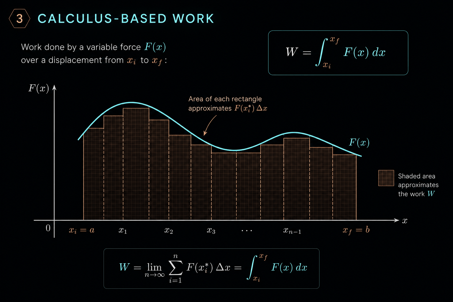
Constant forces are an introductory fiction. Out in the real world, systems rarely experience uniform vectors over a distance. If you track an accelerating interstellar probe, a collapsing star, or a simple macroscopic mechanism, you are tracking forces that evolve continuously with respect to position. When you transition from a flat algebraic product to a variable field, the definition of work must scale from simple arithmetic to a path-dependent line integral.

Mathematically, you define the work done by a variable force vector $\mathbf{F}(\mathbf{r})$ as it moves an object along a parameterized spatial curve $C$ from an initial position $r_i$​ to a final position $r_f​$ as a line integral:

This formulation treats the path as an infinite sequence of differential displacement vectors, $dr$. At each coordinate along the trajectory, you evaluate the inner product of the local force vector and the directional slice of the path. If you are accustomed to calculating the transition amplitudes of a quantum state across a path integral, you will recognize this line integral as the exact classical counterpart. You are summing the localized projections of a vector field along a specific trajectory through configuration space.

To see this operation in a clear one-dimensional scenario, look at the physical mechanics of a standard Hooke's Law spring. When you deform an ideal spring, the restoring force it exerts is not constant. The force scales linearly with displacement, pointing in the opposite direction of the deformation vector:

Here, $k$ is the spring constant, measuring the rigidity of the system. If you want to calculate the work done by an external agent to compress this spring from an initial deformation $x_i$​ to a final position $x_f​$, you substitute this variable force directly into the one-dimensional version of your line integral. The vector notation drops away because the motion and the force are entirely collinear along the $x$-axis:

Evaluating this definite integral requires basic power-rule integration. The antiderivative of $kx$ is $\frac{1}{2}kx^2$. When you evaluate this function at your boundary conditions, the exact work required to alter the spring's state emerges directly from the calculus:

This quadratic dependence on position means the energy requirement scales aggressively the further you push the system out of its equilibrium state.

You can visualize this entire integration process geometrically. If you plot the force vector magnitude on the vertical axis against the position coordinate on the horizontal axis, the resulting function forms a straight line passing through the origin with a slope equal to k. The work done on the system is the exact geometric area under this Force vs. Position curve between your integration limits. For a compression starting from the origin ($x_i​$=0), this area forms a simple right triangle with a base of $x_f​$ and a height of $kx_f​$. The standard geometric area formula for a triangle gives you $\frac{1}{2}$⋅base⋅height, which yields $\frac{1}{2}kx_f^2$. The calculus matches the geometry perfectly.

Consider an explicitly fictional example to ground this geometric area in a physical system. Imagine an industrial testing laboratory in Bengaluru where engineers are calibrating a heavy-duty steel buffer spring used in railway switching yards. They mount the spring into a hydraulic press that tracks the force profile in real-time. If the machine plots a erratic force curve due to a structural defect in the steel alloy, the engineers cannot use the simple triangle area formula to find the energy storage. They must program the data logging system to execute a numerical Riemann summation of the recorded data points. They break the erratic curve into thousands of tiny vertical rectangles, calculating the area of each individual slice, and summing them up to find the total work. Whether the curve is a clean linear line or a highly irregular polynomial, the physical rule remains absolute. The total mechanical energy transferred into that steel spring is identical to the spatial area bounded by the force function and the displacement axis.

When you analyze this from the perspective of an EigenState article, you see that the calculus-based definition of work changes how you perceive force entirely. Force is no longer just an instantaneous push that you measure with a spring scale. It is a spatial distribution. By integrating that distribution along a geometric path, you strip away the explicit time parameter completely and isolate how a field alters the energy state of a particle based purely on its coordinates in space. This spatial accumulation of force is the foundational calculus step required to derive the macroscopic conservation laws that govern the physical universe.

Deriving Translational Kinetic Energy

Every physics textbook presents translational kinetic energy as an introductory fact, but it is actually a mathematical consequence of how you track forces across space. If you are used to analyzing the kinetic energy operator in quantum mechanics by taking the second spatial derivative of a wave function, you know that the classical form must emerge cleanly from macroscopic mechanics. You can arrive at this formulation through two distinct paths: a constant-force algebraic shortcut or a variable-force calculus proof.

The algebraic approach starts by tracking a constant net force acting on a point mass m along a straight path. You begin with the standard kinematic relationship that links initial velocity $v_i$​, final velocity $v_f$​, constant acceleration a, and spatial displacement $x$:

You can isolate the acceleration parameter by rearranging this equation into a purely kinematic ratio:

To inject dynamics into this geometric equation, you substitute this acceleration directly into Newton's second law, $F=ma$. This gives you a direct mathematical statement for the constant force required to cause that specific change in velocity:

If you multiply both sides of this equation by the displacement $x$, you isolate the mechanical work expression on the left side. The spatial parameter cancels out on the right side, forcing the fractional coefficients to distribute cleanly across the mass and velocity terms:

Because $W=Fx$ for a constant parallel force, the work done on the object maps directly to the difference between two states of a new scalar property. This specific grouping of mass and squared velocity is what you define as translational kinetic energy.

This algebraic shortcut works for introductory homework problems, but it falls apart if the acceleration vector fluctuates by even a fraction of a degree. To make the derivation rigorous for the EigenState platform, you must rebuild this proof from the ground up using variable-force calculus. You start with the fundamental definition of work as a one-dimensional integral of a position-dependent force field:

You can replace the force term with its dynamic definition, tracking the instantaneous time rate of change of momentum for a constant mass, which is $F=m\frac{dv}{dt}$​:

This integral looks problematic on its face because you are trying to integrate a time derivative with respect to a spatial coordinate. To resolve this mismatch without introducing complex coordinate transformations, you apply the chain rule to the differential terms. You can mathematically swap the denominators because the time parameter underlies both the changing position and the changing velocity:

Because the time derivative of position is the definition of instantaneous velocity ($v=\frac{dx}{dt}$), this differential manipulation simplifies into a clean, velocity-dependent expression:

This variable shift alters your entire integration landscape. You substitute this identity back into your work integral, which changes your limits of integration from initial and final spatial coordinates to your initial and final velocity states, $v_i$ and $v_f$​:

The mass m acts as a constant scalar multiplier, letting you pull it outside the integral operator. This leaves you with the task of integrating the velocity variable $v$ with respect to itself, which yields the standard antiderivative $\frac{1}{2}v^2$. When you evaluate this primitive function at your upper and lower boundary limits, the final structure appears exactly as it did in the algebraic derivation:

Consider an explicitly fictional example to illustrate how this calculus transformation prevents engineering failures. Imagine a team of aerospace diagnostics engineers working at a launch pad facility near Cape Canaveral. They are analyzing the emergency braking catch-nets designed to arrest a runaway crew transport vehicle if its mechanical brakes fail on a steep access ramp. The resistive force of the catch-net varies drastically as the vehicle deforms the mesh fabric, meaning the force function looks like a complex polynomial rather than a clean constant line. If the tracking software tried to compute the vehicle's terminal velocity using the simple algebraic formula, it would drastically underestimate the required stopping distance. The diagnostic system must constantly track the changing velocity states through the chain-rule integration step, mapping the incoming stream of $v$ $dv$ differentials to ensure the kinetic energy of the vehicle matches the spatial capacity of the net.

This exact mathematical transition from tracking time to tracking space is what gives kinetic energy its utility. By using the calculus derivation, you prove that no matter how chaotic or non-linear the force profile is during a physical event, the total energy shift is entirely determined by the boundary states of the mass. The exact path the velocity takes through time becomes irrelevant because the spatial integration forces the system to conform to this specific quadratic scalar value.

The Work-Energy Theorem (Net Work)

The integration of force over space leads directly to the core operational principle of classical dynamics: the Work-Energy Theorem. If you are accustomed to treating physical states through operator algebra, you can view this theorem as the macroscopic equivalence relation that links kinematic observables to dynamic inputs. It states that the net work executed by every concurrent force acting on a point particle matches the precise variation in that particle's kinetic energy state:

This expression acts as a total accounting system for the object's energy state. You do not get to pick and choose which forces enter the equation on the left side. Whether a force originates from an engineered mechanical linkage, an invisible gravitational field, or dissipative surface interactions, its spatial line integral must be summed into the net work term.

To make this accounting useful for complex systems, you must categorize your forces based on their path dependency. You split the net work parameter into two fundamentally distinct algebraic components: conservative work and non-conservative work:

Conservative forces possess a unique property that you can identify instantly if you are familiar with vector calculus. The curl of a conservative force field is identically zero $(\nabla \times \mathbf{F} = 0)$, which means the line integral of this force around any closed loop vanishes completely. Because the work done by a conservative field depends solely on the initial and final coordinates, you can bypass path integrals entirely by defining a spatial scalar field called potential energy, $U(r)$. You mathematically define this potential energy state such that the work done by the conservative field is equal to the negative variation in potential energy:

When you substitute this potential identity back into your split work equation, the underlying structure of energy conservation emerges. You replace $W_{\text{net}}$​ with $\Delta K$ and isolate the non-conservative terms on one side of the relation:

By expanding the delta terms into their explicit initial and final states $(K_f​−K_i​=−U_f​+U_i​+W_{\text{non-cons}})$ and grouping all initial parameters on the left side, you reformulate the Work-Energy Theorem into the generalized law of conservation of mechanical energy:

Here, $E$ represents the total mechanical energy of the system, defined simply as the sum of its kinetic and potential states $(E=K+U)$. If your non-conservative work term drops to zero, the total mechanical energy at the start matches the final energy state exactly, creating a pristine invariant.

Consider an explicitly fictional example to illustrate how this partitioning prevents critical miscalculations when non-conservative forces dominate the system. Imagine an automotive testing track in the dry terrain near Chennai where engineering teams are evaluating the emergency runaway ramps designed for heavy freight trucks. A massive multi-axle truck loses its hydraulic brakes on a steep decline and veers into the runaway ramp, which consists of an inclined path filled with a deep, uniform layer of loose gravel. If the safety software only accounts for the conservative force of gravity $(W_{\text{cons}})$, it would predict that the truck will slide up the incline, stop, and then slide backward down the ramp like an ideal pendulum. The software must track the non-conservative work ($W_{\text{non-cons}}$​) performed by the high-friction gravel bed, which actively drains mechanical energy from the truck by converting it into displacement of the stones and localized thermal energy. The gravel bed performs massive negative non-conservative work, ensuring that the final mechanical energy $E_f$​ drops to a state where the truck comes to a permanent, static halt at the top of the ramp.

From the perspective of your writing on the EigenState platform, this mechanical partition provides a direct conceptual line to advanced field theories. You are witnessing the classical foundation of how constraints and potentials govern the behavior of matter. When you transition from this classical accounting system to quantum mechanics, you stop tracking the explicit non-conservative work term directly. Instead, you absorb these dissipative interactions into external potentials or couple the particle to an environmental bath of infinite degrees of freedom. The foundational tracking system remains identical: you are mapping how external inputs alter the fundamental energy eigenvalues of your system across space.

Rotational Kinetic Energy and Moment of Inertia

An object does not need to traverse a spatial path across your laboratory to possess kinetic energy. A stationary flywheel spinning about its geometric center has zero net linear momentum, yet it contains a massive reservoir of energy. If you look at this through the lens of quantum mechanics, you will recognize it as the classical equivalent of orbital angular momentum operators acting on a rigid state vector. The system's center of mass remains perfectly static, but each individual mass element inside the object is locked in an instantaneous state of translational acceleration.

To derive this rotational kinetic energy formally, you begin by conceptually slicing an arbitrary rigid body into an infinite assembly of discrete, microscopic mass elements denoted by $m_i$​. Each individual element occupies a specific position coordinate at a perpendicular distance $r_i​$ from the fixed axis of rotation. As the rigid body spins with a uniform angular velocity $\omega$, every internal mass slice moves with an instantaneous tangential linear velocity $v_i$​. You convert this linear velocity into its angular counterpart using the fundamental geometric transformation:

You can now express the total kinetic energy of the rotating object as the discrete summation of the translational kinetic energies of all these microscopic mass elements. By substituting your angular velocity identity into the standard kinetic energy equation, you structure the summation across the entire volume of the object:

Because the object is rigid, every mass element shares the exact same angular velocity $\omega$ regardless of its distance from the pivot. This spatial invariance allows you to factor both the fractional coefficient $\frac{1}{2}$ and the squared angular velocity parameter $\omega^2$ completely outside the summation operator:

The algebraic term isolated within the parentheses is the moment of inertia, $I=\sum m_i ​r_i^2​$. For continuous macroscopic systems, you transition this discrete sum into a volume integral over the mass density distribution, $I=\int r^2 dm$. This value represents the structural resistance of a system to angular acceleration, functioning as the exact rotational counterpart to inertial mass. Replacing the parentheses with this defined property gives you the definitive rotational energy equation:

Calculating this inertial parameter becomes more involved when the rotation axis shifts away from the object's center of mass. To evaluate these non-standard states on the EigenState platform without re-running entire volume integrals, you use two fundamental geometric theorems. The Parallel Axis Theorem lets you find the moment of inertia $I$ about any axis parallel to a known axis passing through the center of mass, using the object's total mass $M$ and the perpendicular displacement distance d between the two axes:

The Perpendicular Axis Theorem applies strictly to planar objects, stating that the moment of inertia about a perpendicular axis z matches the direct sum of the moments about the two orthogonal axes lying within the plane of the object ($I_z​=I_x​+I_y$)

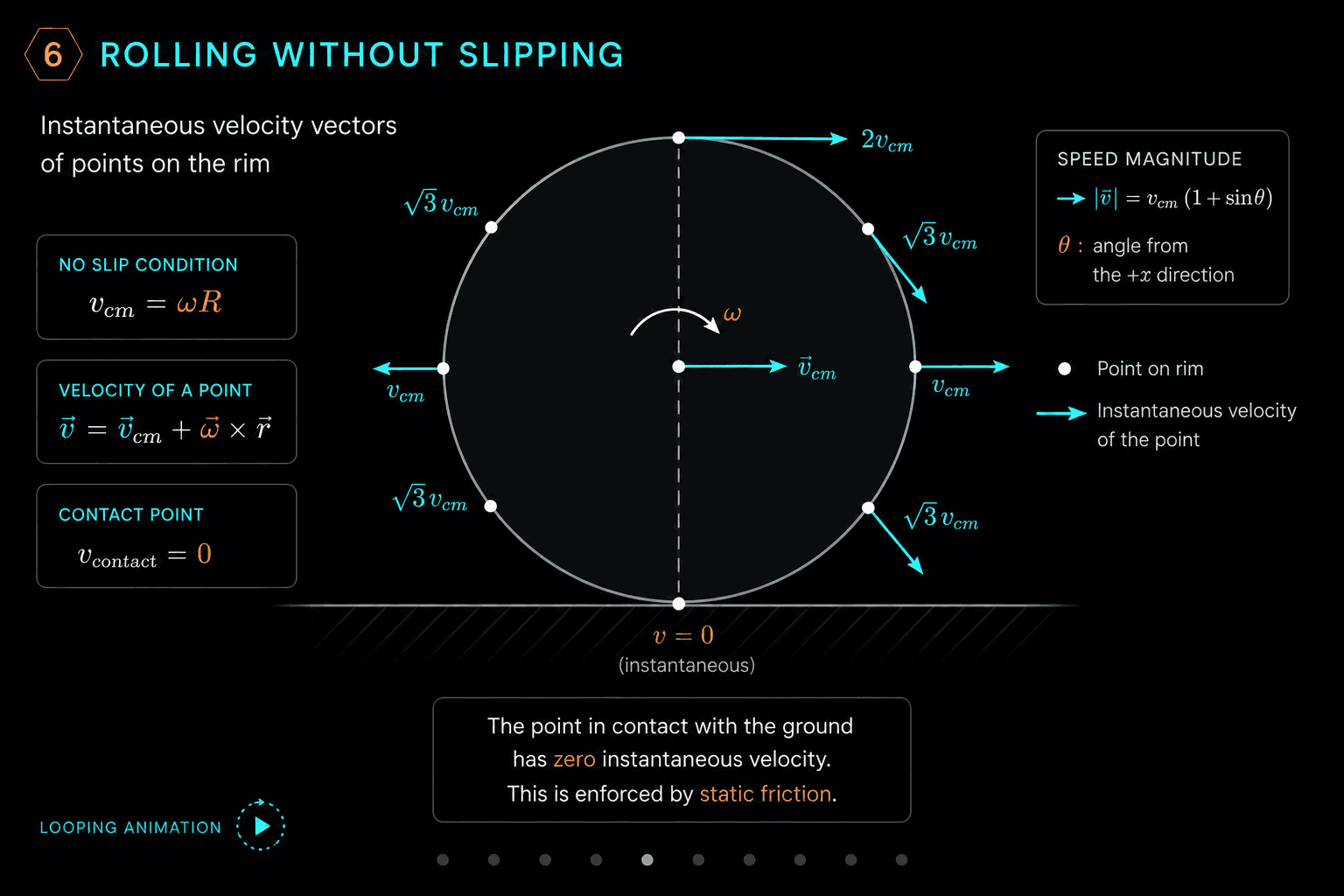
When an object rolls smoothly across a flat surface without slipping, you are tracking a combined mechanical state where translation and rotation exist simultaneously. You cannot treat these motions as isolated phenomena. Instead, you express the total kinetic energy of the system as the clean addition of its linear center-of-mass energy and its rotational energy relative to that center of mass:

Because the rolling motion satisfies the zero-slip boundary condition, the linear velocity maps directly to the angular velocity via $v_{\mathrm{cm​}} = \omega R$, where $R$ is the outer radius of the object. This constraint couples the two energy terms together, forcing the total distribution of energy to depend entirely on how the object's mass is distributed relative to its geometric center.

Advanced Applications and Systems of Particles

To scale your energy accounting from single rigid bodies to complex multi-particle systems, you must track how kinetic energy distributes across an assembly of $N$ separate interacting particles. If you study multi-body quantum mechanics or quantum statistical fields, you are already accustomed to managing the total kinetic energy operator by summing over the individual Laplacian operators for every particle in the configuration space.

In classical mechanics, you formalize this collective behavior through König’s Theorem. This decomposition theorem states that the total kinetic energy of any multi-particle system can be split cleanly into two independent components: the translation of the collective center of mass and the internal kinetic energy of the particles measured relative to that center of mass frame.

Mathematically, you define the position of the $i$-th particle as $r_i​=R{\mathrm{cm​}}+r_i′​$, where $R{\mathrm{cm​}}$​ is the vector locating the system's center of mass and $r_i′$ is the particle's relative position vector within the center-of-mass frame. Taking the time derivative yields the velocity relation $v_i​=V{\mathrm{cm​}}+v_i′​$. When you substitute this velocity vector into the total kinetic energy summation for all particles, the algebraic expansion forces a cross-product term to appear:

The third term on the right side contains the expression $\sum m_i ​v_i′$​, which represents the total linear momentum of the system calculated strictly inside the center-of-mass reference frame. By definition, the net momentum in the center-of-mass frame is identically zero, causing that entire cross-term to vanish. The remaining terms give you the definitive statement of König’s Theorem:

This algebraic decomposition means you can analyze the external trajectory of a complex, exploding system as if it were a single point mass $M$, while completely separating the internal thermal or chaotic kinetic energies of its components.

This multi-particle tracking is what allows you to evaluate macroscopic collisions. When two independent bodies interact through a collision event, the conservation of total linear momentum holds absolute because external forces are zero over the short interaction window. However, the total kinetic energy of the system behaves differently depending on the internal material properties of the colliding objects.

In an ideal elastic collision, the total kinetic energy of the system is a conserved invariant. The initial kinetic energy state matches the final state perfectly ($K_i​=K_f$​), meaning no energy is diverted into altering the internal structures of the masses. If you model low-energy gas particles colliding inside a vacuum chamber, they approximate this elastic behavior.

Once you look at macroscopic objects, collisions become inelastic. While momentum remains conserved, total kinetic energy drops during the impact ($K_f​<K_i​$). In a perfectly inelastic collision, the two objects stick together completely after the impact, moving forward with a single shared final velocity.

Consider an explicitly fictional example to ground this energy loss in a real-world scenario. Imagine an automotive crash-testing facility located off a highway near Detroit. Engineers are accelerating a structural steel test chassis down a track to slam it into a stationary concrete barrier at high speed. The telemetry sensors show that the system's total kinetic energy drops sharply to zero the instant the chassis strikes the wall. Because kinetic energy cannot simply vanish from the universe, the lost energy is violently redirected. The bulk of that kinetic scalar currency is consumed by non-conservative work during the permanent plastic deformation of the steel frame, bending columns and crumpling impact zones. The remaining energy propagates out into the environment as an acoustic pressure wave—the loud bang of the impact—and a sudden spike in localized thermal energy across the twisted metal joints. The kinetic energy changes its form entirely, leaving the macro-system trapped in a static, deformed state.

Relativistic Corrections: When Newton Fails

The quadratic simplicity of $\frac{1}{2}mv^2$ is an approximation that holds only when an object stays anchored to the slow speeds of the macroscopic world. If you track particles accelerated within interstellar fields or high-energy physics laboratories, the Newtonian framework collapses entirely. As a velocity vector approaches the speed of light ($c$), the energy required to achieve a further incremental increase in velocity approaches infinity. You cannot use classical mechanics to decode these high-velocity states because mass and velocity do not scale linearly near the speed of light.

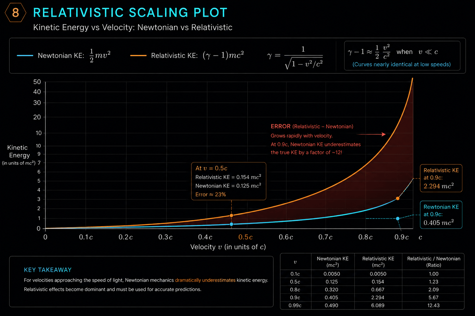
To correct these equations for the EigenState platform, you must introduce the Lorentz factor, denoted by the Greek letter $\gamma$. This dimensionless scaling factor accounts for the relativistic transformations of spacetime coordinates:

As velocity $v$ approaches zero, $\gamma$ approaches 1. As $v$ approaches $c$, $\gamma$ approaches infinity. This scaling factor alters how you define linear momentum. The classical expression $p=mv$ must be replaced with the relativistic momentum vector, which incorporates this non-linear scaling:

To derive the actual expression for relativistic kinetic energy, you must return to the fundamental calculus-based definition of work. You integrate the net force over a distance, but you swap out the Newtonian force with the relativistic definition of force, which is the time derivative of relativistic momentum ($F = \frac{dp}{dt}$):

Applying the same chain-rule differential swap you used in the classical derivation allows you to rearrange the spatial and temporal differentials ($\frac{dx}{dt}=v$). This shifts the integration variable from position to velocity, bounded by your initial static state and your final relativistic velocity:

Evaluating this integral requires integration by parts or a direct substitution of the explicit $\gamma$ function. When you carry out the integration across these relativistic boundary conditions, the expression resolves into a clear difference between the total energy of the moving particle and its baseline rest energy:

This is the definitive equation for relativistic kinetic energy. It looks completely alien compared to the Newtonian expression. There is no explicit velocity squared term visible in the core structure; the velocity dependency is buried entirely within the denominator of the Lorentz factor.

To prove that this formula is not disconnected from classical mechanics, you can apply a Taylor series binomial expansion to the Lorentz factor. You expand $\gamma$ as a polynomial series centered around the low-velocity limit where the ratio $\frac{v}{c}$ is much less than 1 ($v \ll c$):

Now, substitute this infinite polynomial expansion back into your relativistic kinetic energy formula:

The leading constant 1 and the trailing negative 1 cancel each other out completely. You then distribute the rest-energy scalar $mc^2$ across the remaining terms of the truncated series:

When $v$ is exceptionally small compared to c, every higher-order term beyond the first fraction becomes so microscopically small that it vanishes for all practical purposes. The infinite series collapses, leaving you with exactly $\frac{1}{2}mv^2$. The Newtonian formula is revealed to be nothing more than the first-order approximation of a deeply non-linear relativistic reality.

Conceptual Edge Cases, Misconceptions, and Paradoxes

Even within low-speed classical mechanics, the Work-Energy Theorem harbors subtle conceptual traps that can easily confuse an ungrounded analysis. The first trap involves the frame of reference dependency of kinetic energy. Velocity is not an intrinsic property of matter; it is a coordinate-dependent measurement that changes based on your chosen Galilean reference frame.

Consider an explicitly fictional example where a passenger is sitting completely still in a seat on an Amtrak train accelerating out of a station in Chicago. An observer standing static on the station platform looks through the window and calculates that the passenger has a massive, rapidly increasing kinetic energy state because the train is moving at high speed. Meanwhile, a second observer sitting directly across the aisle from the passenger calculates their kinetic energy to be exactly zero because their relative velocity vector is null.

This mismatch looks like a physical paradox, but it resolves perfectly when you apply the Work-Energy Theorem consistently across independent Galilean frames. The observer on the platform tracks the positive work done on the passenger by the forward macroscopic force of the seatback over a measurable spatial distance. The observer on the train tracks zero displacement inside their moving coordinate system, meaning the net work done on the passenger in that specific frame is exactly zero. Both frames yield completely different absolute numbers for work and energy, yet the relationship $\Delta K=W_{\text{net}}$ holds true in every single inertial frame. Energy shifts are frame-dependent, but the causal law linking force replication to energy alteration remains invariant.

The second major point of confusion centers around the static friction paradox. A common misconception states that because static friction requires zero relative slipping between contacting surfaces, it can never execute mechanical work. This assumption falls apart when you look at how a system accelerates from a standstill.

When you step onto a concrete walkway, your foot pushes backward against the ground, and the ground pushes your foot forward with an equal and opposite force of static friction. Because your foot does not slip against the concrete during the push, the instantaneous displacement of the point of contact is zero. However, if you treat your entire human body as a composite system of interacting mass segments rather than a rigid point particle, the static friction force acts as an external constraint that allows your internal muscular forces to shift your collective center of mass forward over a finite distance. The static friction force does real, positive work on your body's center of mass, translating internal chemical energy into macro-system kinetic energy. The same mechanism applies to a car accelerating along a paved road; the static friction between the tire tread and the asphalt is the precise external vector that pushes the vehicle's mass forward.

Finally, you must separate how internal forces alter the different layers of a multi-particle system's energy structure. An internal force is an interaction that originates and terminates entirely within the defined boundaries of your system. According to Newton’s third law, these internal forces always appear in balanced, opposing pairs, which means their vector sum is identically zero. Because the net internal force vanishes, internal interactions cannot alter the total linear momentum of the system, nor can they change the translational kinetic energy of the collective center of mass.

However, these internal forces can execute massive work within the system's internal coordinate space, violently altering the total internal kinetic energy. Think about a firework shell coasting through a predictable parabolic trajectory in the night sky. When the internal gunpowder core ignites, the chemical explosion unleashes massive internal forces that push the metallic fragments outward in every direction. The collective center of mass of the exploding fragments continues to coast along the exact same pre-explosion parabolic path as if nothing happened, completely unaffected by the blast. Yet, the internal kinetic energy of the system has spiked drastically. The internal forces converted static molecular potential energy into the chaotic, high-velocity kinetic motion of a thousand glowing fragments. You are witnessing a complete redistribution of internal states achieved without a single Newton of external force acting upon the system.